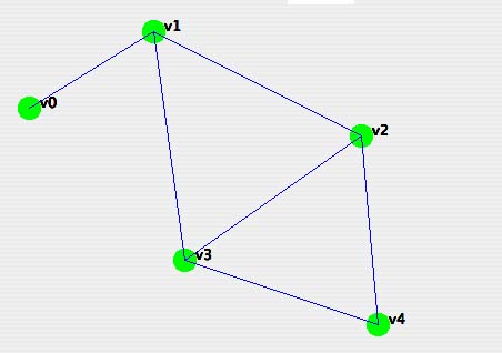
Graph convolutional networks are in general known as message passing network. They are used generally in a graph G(V,E) where nodes or vertices are properly connected with each other and the connections are shown by node edges just like below figure.
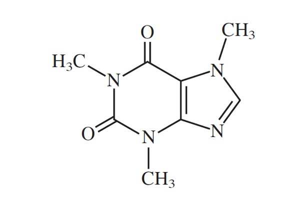
A very popular and easy to understand example would be a chemical molecule where each atom is considered as a node and the chemical bonds are considered as edges.
In Graph Neural Networks, there are two types of features involved.
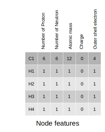
- Node features: This type of features describe the characteristics of a node. So, each node is represented by its corresponding node feature. For the molecular example, the node feature space may contain atomic number, atomic mass, number of electrons, charge value, chiral center or not etc. information regarding an atom.
- Edge features: The connection between two atoms are represented by edge feature. In a plain graph G(V,E), this edge feature might just be a 1/0 value indicating the connection is present or not. But in molecular example, it might express more information like the type of the bond between two atoms, explicit bond information in a multi-dimensional feature space.
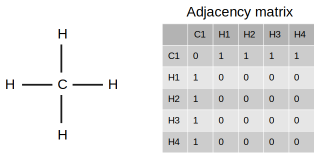
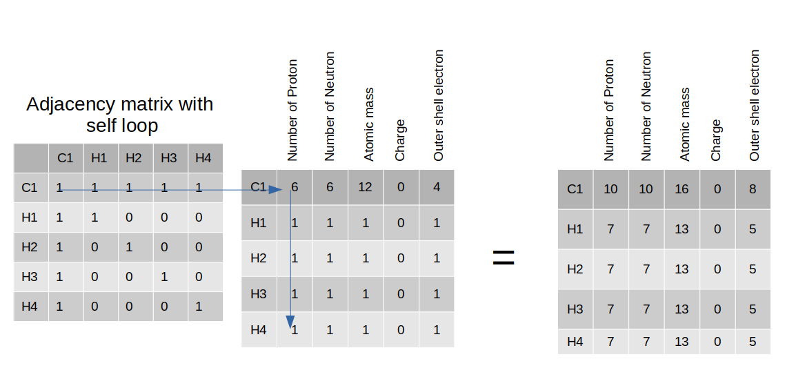
There is also another term named as 'Adjacency Matrix' which represents the connection of nodes in a matrix format. For example, if we have a molecule of methane CH4, we can construct a matrix of size 5x5 to indicate the connection between each pair of atoms.
The corresponding node features may be represented by this table-
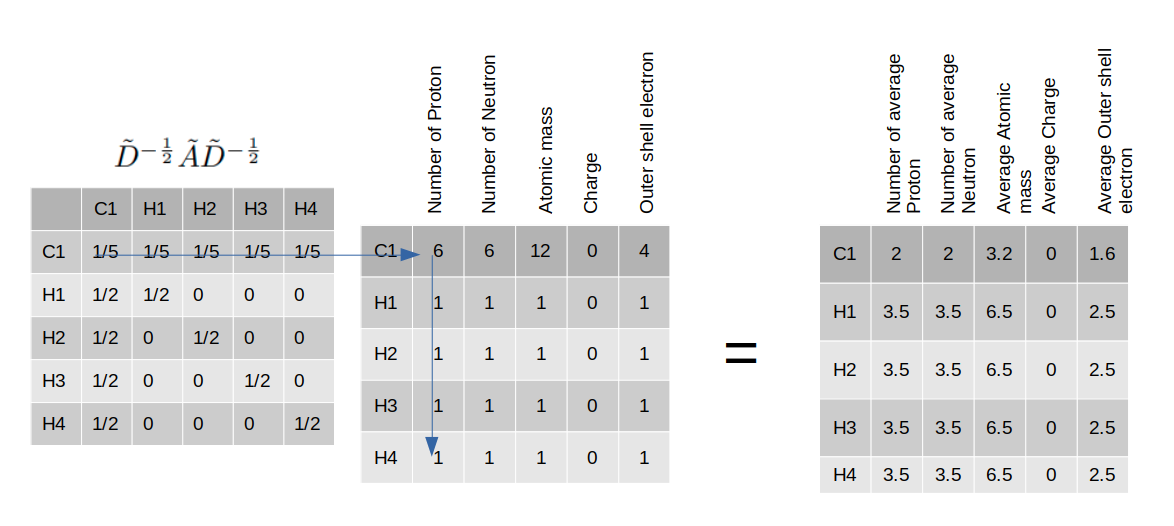
This is the node processing formula for a Graph Convolutional Network
A few things happening here all at once
- This equation is multiplying adjacency matrix with the feature vectors of connected nodes only.
- The identity matrix added to the adjacency matrix is adding extra 1 at all diagonal entries so that during multiplication of step-1, the features of node itself are also considered.
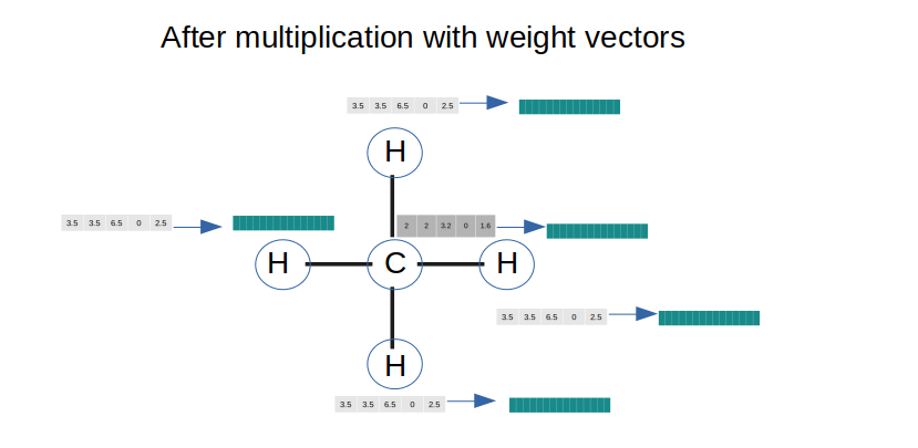
This computation will be applied to all nodes of the graph. Finally, we can get new node feature vectors for all nodes
- Each time the node feature is processed, the corresponding node gets information about its adjacent nodes only.
- If we want the node to get information about further nodes, we need to add more convolutional layers.
- Basically, each convolution operation get information of depth = 1. So, for reaching a depth of 3, we need to apply three cascaded graph convolution.
- We can use activation and normalization operations between convolution operations if we want.
- for a fully connected graph where all nodes are connected to each-other, one convolutional layer is enough.
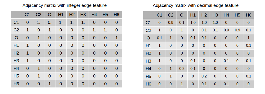
So far, we have seen only the representation of node features. But, edge feature is also important information in a Graph. Edge feature is already used in above calculation inside the adjacency matrix where we put one to show node connections. But in a generalized way, this computation can be modified by introducing decimal values instead of putting exact 1. This way, we can show how strong the connection/bond is between two nodes.
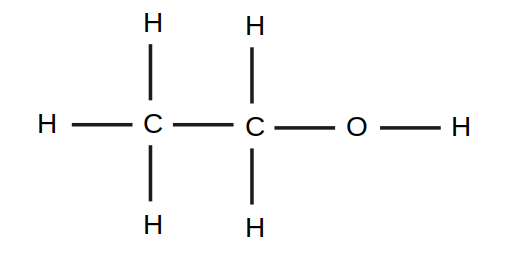
But, it needs more generalization. Lets assume, we have a molecule of CH3-CH2-OH where there are different types ob bonds such as C-C bond, C-H bond, H-H bond, C=O bond etc. S, to represent these different types of bonds we need to introduce one hot vectors. So, now we can not accommodate all values of these bond type feature inside the adjacency matrix. So, directly Graph Convolution can not be applied using edge features.
A few things are happening in this equation to process the features of node
- concatenate node features of two node ends (
$X_i$ ,$X_j$ ) where$X_j$ is feature of a neighboring node of$X_i$ and edge features$e_{ij}$ together - process the combined features through a Fully connected (Linear/Dense)
- repeat this for all neighboring nodes of
$X_i$ - get average/sum or any other pooling mechanism to get a feature vector from all the neighboring features
- concatenate the processed feature with the actual node feature of
$X_i$ - process with another fully connected layer to get final feature representation of the node feature of
$X_i$
After processing the node features, we can also update the edge features using another fully connected layer for only edge feature processing. We can use updated node features here so that
So basically, we can concatenate updated node features of two ends of an edge and the old edge feature and then process them through a FCN layer.
According to the implementation available on torch_geometric library, they do not allow edge feature processing in GCN layer. That's why in the code, I used Graph Attention network to process edge features.But you can still use MessagePassing layer from torch_geometric because it allows edge feature processing.
In torch_geometric, the molecule methane (CH4) will be explained by a graph and to construct the graph, we need ot define the nodes and their connections.
We can do it this way-
- Lets define indices of the atoms as 0, 1, 2, 3, 4 for C, H1, H2, H3, H4 respectively
- Define the edges in a 8x2 matrix (8x2 because for each edge, there will be 2 node indices and for undirected edge, we have to define it both way (i, j) and (j, i))
- Define the features in a 5x5 matrix (5 atoms, 5 features)
- Use torch_geometric.data.Data class for these definitions
- Edge features can be defined in Data class object using argument 'edge_attr'
- label can be defined in Data class object using argument 'y'
We can look at the piece of the code below to do that-
# definition of methane
# CH4
edge_index = torch.tensor(
    [[0, 1], [1, 0],
     [0, 2], [2, 0],
     [0, 3], [3, 0],
     [0, 4], [4, 0]], dtype=torch.long)

# calling continguous() is necessary here
edge_index = edge_index.t().contiguous()

# description of features
# #proton, #neutron, atomic mass, charge, outer shell electrons
x = torch.tensor(
    [[6, 6, 12, 0, 4],
     [1, 1, 1, 0, 1],
     [1, 1, 1, 0, 1],
     [1, 1, 1, 0, 1],
     [1, 1, 1, 0, 1]], dtype=torch.float)

# lets assume edge feature is distance between two atoms
# for 4 edges, we had to define 8 edge_index entries. So, similarly, we need to define 8 feature values with shape (8, 1).
# We can repeat avialable 4 values to fulfill 8 values
edge_feature = torch.tensor([[1.5, 1.5, 2.4, 2.4, 1.6, 1.6, 1.3, 1.3]]).T

# label: lets imagine label is binary whether the molecule is organic or not. Methane is organic so 1
y = torch.tensor(1)

# data definition
from torch_geometric.data import Data
molecule = Data(x=x, edge_index=edge_index, edge_attr=edge_feature, y=y)
molecular Energy prediction from molecular graph. Label was provided an energy values for each molecule in the data set. As energy values are decimal values, regression model was used to predict.
data is downloaded from kaggle website (https://www.kaggle.com/c/champs-scalar-coupling)
- Node and edge features were extracted from the molecular structures.
- For each node, I have calculated these features- ['proton', 'neutron', 'mass', 'outer_electron', 'outer_electron_def', 'total_shell']
- For each edge/bond, bond-type feature was provided in the dataset. So, it was used in one-hot encoded format. atomic distance between two atoms inside a molecule was calculated from molecular structure information. This was another edge feature. The last edge feature was scalar-coupling-constant value provided in the training data only (this is the main label of the kaggle competition).
- Only training data (train.csv) from the provided kaggle data set was used for train, validation and test.
- Provided training data was split into 70-15-15 split respectively.
- Data processing takes much time. So, its suggested to run the script 'src/prepare_data.py' separately
- After that, training and evaluation can be done using 'src/train.py'
- Prepare a virtual environment and install all necessary libraries from requirements.txt (if you face issues regarding installation of torch_geometric, please refer here- https://pytorch-geometric.readthedocs.io/en/latest/install/installation.html)
- Check system requirements of pytorch from https://pytorch.org/ and install pytorch properly
- Download data from kaggle and set parameters in config.py properly including the data directory path
- open terminal from this directory where README.md is kept and run the command
python src/prepare_data.py --problem-type=energy-prediction --save-path=output_energy - run training using the command
python src/train.py --problem-type=energy-prediction --save-path=output_energy
Note that the modeling was done for demonstration purposes only. So, the results are not very impressive. Also, the processing code can be optimized in many ways for faster processing which is out of scope for this demonstration.
atomic bond prediction in the molecular graph. Label was provided as bond type values for each bond the molecule in the data set. As bond type values are categorical values, multi-class classification model was used to predict.
Same as energy prediction except that energy data was not necessary for this experiment.
- Node and edge features were extracted from the molecular structures.
- For each node, I have calculated these features- ['proton', 'neutron', 'mass', 'outer_electron', 'outer_electron_def', 'total_shell']
- For each edge/bond, bond-type value was provided in the dataset. It was converted to indices as pytorch can only allow index for multi-classification label.
- Used bondtypes are ['1JHC', '2JHH', '1JHN', '2JHN', '2JHC', '3JHH', '3JHC', '3JHN']. These were replaced by indices as 0, 1 2, ...
- Atomic distance between two atoms inside a molecule was calculated from molecular structure information. This was one edge feature. Another edge feature was scalar-coupling-constant value provided in the training data only (this is the main label of the kaggle competition).
- Only training data (train.csv) from the provided kaggle data set was used for train, validation and test.
- Provided training data was split into 70-15-15 split respectively.
- Data processing takes much time. So, its suggested to run the script 'src/prepare_data.py' separately
- After that, training and evaluation can be done using 'src/train.py'
- Prepare a virtual environment and install all necessary libraries from requirements.txt (if you face issues regarding installation of torch_geometric, please refer here)
- Check system requirements of pytorch from https://pytorch.org/ and install pytorch properly
- Download data from kaggle and set parameters in config.py properly including the data directory path
- open terminal from this directory where README.md is kept and run the command
python src/prepare_data.py --problem-type=bond-prediction --save-path=output_bondtype - run training using the command
python src/train.py --problem-type=bond-prediction --save-path=output_bondtype
Note that the modeling was done for demonstration purposes only. So, the results are not very impressive. Also, the processing code can be optimized in many ways for faster processing which is out of scope for this demonstration.
- Torch-geometric webpages:
- Installation: https://pytorch-geometric.readthedocs.io/en/latest/install/installation.html
- Introduction: https://pytorch-geometric.readthedocs.io/en/latest/get_started/introduction.html
- Data class: https://pytorch-geometric.readthedocs.io/en/latest/generated/torch_geometric.data.Data.html#torch_geometric.data.Data
- DataLoader: https://pytorch-geometric.readthedocs.io/en/latest/modules/loader.html
- Youtube explanatory example: https://www.youtube.com/watch?v=VXFFHHoE1wk
- Github explanatory example: https://github.com/masashitsubaki/molecularGNN_smiles
- Dataset links:
- Edge prediction and edge feature utilization:
- Relevant papers
- initial idea of graph convolution and message passing (https://arxiv.org/abs/1509.09292)
- Neural Message Passing Network paper (https://arxiv.org/abs/1704.01212v2)
- Graph Convolutional Network paper (https://arxiv.org/abs/1609.02907)
- Graph Attention Network paper (https://arxiv.org/abs/1710.10903)
- Mathematical expressions in markdown (https://rpruim.github.io/s341/S19/from-class/MathinRmd.html)
- msdlib resources
- documentation https://msdlib.readthedocs.io/en/latest/
- github repository https://github.com/abdullah-al-masud/msdlib
