FINAL PROJECT DRAFT
What: For my final project, I originally wanted to find out the cost of health care in us prior covid and post covid to determine if COVID-19 has affected the price of healthcare at all or not and by how much compare to the previous years. But after looking for a data set, I could not really find what I needed, so I have decided to put my focus on the national spending on healthcare to analyse the amount on money spent on hospital, home_healthcare,personal healthcare, money paid out of pocket and private insurance from 1960 to 2020. So I have decided to analyze the data to see if there is any significant increase or decrease in the spending since 1960 and if there is a correlation between year and each category.
Why: I think it would be interesting to see if there is any increase or decrease over time in each categories of spending and possibly find events that may have impacted them.
How: I will try to explore datasets about national spending on healthcare and expenditure cost and use R studio to make analysis and visualization that show spending over time and how much money spent on healthcare.
Minimal scenario: I explore the datasets but find there is no change in the spending over time.
Optimistic scenario: I find the datasets and run my analysis and find that there is a substantial change in the spending over time and observe an increase or decrease in each spending category each year since 1960 to 2020
Ambitious scenario: I explore the datasets and find that there is a relationship between years and healthcare spending which prove that healthcare cost will continue to go up or down year after year which increase the spending in each category cited above.
This data set is from the national spending on healthcare. it contains 61 observations and 6 variables that i will use to run my analysis and explains the findings.
library(tidyverse)

## ── Attaching packages ──────────────────────────────────────────── tidyverse 1.3.1 ──

## ✔ ggplot2 3.3.6     ✔ purrr   0.3.4
## ✔ tibble  3.1.7     ✔ dplyr   1.0.9
## ✔ tidyr   1.2.0     ✔ stringr 1.4.0
## ✔ readr   2.1.2     ✔ forcats 0.5.1

## ── Conflicts ─────────────────────────────────────────────── tidyverse_conflicts() ──
## ✖ dplyr::filter() masks stats::filter()
## ✖ dplyr::lag()    masks stats::lag()

library(readr)
nationalspending <- read_csv("nationalspending.csv")

## Rows: 61 Columns: 6

## ── Column specification ─────────────────────────────────────────────────────────────
## Delimiter: ","
## dbl (6): Year, Hospital_spending, Home_health_care ($), Personal_healthcare ($), ...
##
## ℹ Use `spec()` to retrieve the full column specification for this data.
## ℹ Specify the column types or set `show_col_types = FALSE` to quiet this message.

View(nationalspending)
read.csv("nationalspending.csv")

##    Year Hospital_spending Home_health_care.... Personal_healthcare....
## 1  1960        8.9850e+09           5.7000e+07              2.3124e+10
## 2  1961        9.7770e+09           6.1000e+07              2.4624e+10
## 3  1962        1.0432e+10           6.5000e+07              2.6530e+10
## 4  1963        1.1507e+10           6.9000e+07              2.8976e+10
## 5  1964        1.2501e+10           7.5000e+07              3.1825e+10
## 6  1965        1.3545e+10           8.9000e+07              3.4421e+10
## 7  1966        1.5298e+10           1.0800e+08              3.8009e+10
## 8  1967        1.7798e+10           1.6400e+08              4.2989e+10
## 9  1968        2.0537e+10           2.3800e+08              4.8624e+10
## 10 1969        2.3367e+10           2.7200e+08              5.4871e+10
## 11 1970        2.7168e+10           2.2000e+08              6.2369e+10
## 12 1971        3.0224e+10           1.9400e+08              6.8700e+10
## 13 1972        3.3846e+10           2.2000e+08              7.6389e+10
## 14 1973        3.7920e+10           2.7600e+08              8.5344e+10
## 15 1974        4.4139e+10           4.2300e+08              9.7827e+10
## 16 1975        5.1234e+10           6.2300e+08              1.1200e+11
## 17 1976        5.9402e+10           8.9600e+08              1.2800e+11
## 18 1977        6.7023e+10           1.1470e+09              1.4500e+11
## 19 1978        7.5621e+10           1.5560e+09              1.6200e+11
## 20 1979        8.6162e+10           1.8990e+09              1.8500e+11
## 21 1980        1.0100e+11           2.3780e+09              2.1400e+11
## 22 1981        1.1700e+11           2.9380e+09              2.4900e+11
## 23 1982        1.3400e+11           3.4820e+09              2.7900e+11
## 24 1983        1.4500e+11           4.2370e+09              3.0800e+11
## 25 1984        1.5400e+11           5.1290e+09              3.3800e+11
## 26 1985        1.6500e+11           5.6330e+09              3.7300e+11
## 27 1986        1.7600e+11           6.3680e+09              4.0500e+11
## 28 1987        1.9000e+11           6.6360e+09              4.4400e+11
## 29 1988        2.0600e+11           8.4060e+09              4.9500e+11
## 30 1989        2.2600e+11           1.0213e+10              5.4700e+11
## 31 1990        2.5000e+11           1.2534e+10              6.1200e+11
## 32 1991        2.7600e+11           1.5135e+10              6.7300e+11
## 33 1992        2.9800e+11           1.8690e+10              7.2800e+11
## 34 1993        3.1600e+11           2.2748e+10              7.7600e+11
## 35 1994        3.2800e+11           2.7307e+10              8.1800e+11
## 36 1995        3.3900e+11           3.2270e+10              8.6700e+11
## 37 1996        3.5100e+11           3.5716e+10              9.1500e+11
## 38 1997        3.6300e+11           3.6885e+10              9.6600e+11
## 39 1998        3.7500e+11           3.4072e+10              1.0200e+12
## 40 1999        3.9400e+11           3.2756e+10              1.0800e+12
## 41 2000        4.1600e+11           3.2294e+10              1.1600e+12
## 42 2001        4.4900e+11           3.4271e+10              1.2600e+12
## 43 2002        4.8600e+11           3.6465e+10              1.3700e+12
## 44 2003        5.2600e+11           4.0179e+10              1.4800e+12
## 45 2004        5.6500e+11           4.4641e+10              1.5800e+12
## 46 2005        6.0900e+11           4.9343e+10              1.6900e+12
## 47 2006        6.5100e+11           5.2052e+10              1.8100e+12
## 48 2007        6.9200e+11           5.7475e+10              1.9200e+12
## 49 2008        7.2200e+11           6.2165e+10              2.0100e+12
## 50 2009        7.7100e+11           6.6999e+10              2.1100e+12
## 51 2010        8.0900e+11           7.0525e+10              2.1800e+12
## 52 2011        8.3300e+11           7.4623e+10              2.2500e+12
## 53 2012        8.7800e+11           7.8076e+10              2.3500e+12
## 54 2013        9.0700e+11           8.0947e+10              2.4100e+12
## 55 2014        9.4100e+11           8.4647e+10              2.5300e+12
## 56 2015        9.8900e+11           8.9572e+10              2.6700e+12
## 57 2016        1.0400e+12           9.3720e+10              2.8000e+12
## 58 2017        1.0800e+12           9.9440e+10              2.9100e+12
## 59 2018        1.1200e+12           1.0600e+11              3.0200e+12
## 60 2019        1.1900e+12           1.1300e+11              3.1800e+12
## 61 2020        1.2700e+12           1.2400e+11              3.3600e+12
##    Out_of_pocket.... Private_Health_Insurance....
## 1         1.2778e+10                   4.8780e+09
## 2         1.3193e+10                   5.4440e+09
## 3         1.4085e+10                   6.0530e+09
## 4         1.5171e+10                   6.7820e+09
## 5         1.6669e+10                   7.7630e+09
## 6         1.7863e+10                   8.5630e+09
## 7         1.8132e+10                   8.6940e+09
## 8         1.7985e+10                   8.8950e+09
## 9         1.9951e+10                   1.0003e+10
## 10        2.1911e+10                   1.1781e+10
## 11        2.4208e+10                   1.3800e+10
## 12        2.5515e+10                   1.5526e+10
## 13        2.7805e+10                   1.7388e+10
## 14        3.0737e+10                   1.9423e+10
## 15        3.3311e+10                   2.3014e+10
## 16        3.6036e+10                   2.7203e+10
## 17        3.9281e+10                   3.2481e+10
## 18        4.3137e+10                   3.8163e+10
## 19        4.6043e+10                   4.3668e+10
## 20        4.9929e+10                   5.1643e+10
## 21        5.5258e+10                   6.0277e+10
## 22        6.1932e+10                   7.1032e+10
## 23        6.8606e+10                   8.1131e+10
## 24        7.4660e+10                   8.9794e+10
## 25        8.2417e+10                   9.8401e+10
## 26        9.1566e+10                   1.1000e+11
## 27        9.9655e+10                   1.1700e+11
## 28        1.0600e+11                   1.3200e+11
## 29        1.1600e+11                   1.5400e+11
## 30        1.2300e+11                   1.7500e+11
## 31        1.3400e+11                   2.0000e+11
## 32        1.3700e+11                   2.2100e+11
## 33        1.3900e+11                   2.3800e+11
## 34        1.4000e+11                   2.5200e+11
## 35        1.3800e+11                   2.6400e+11
## 36        1.4100e+11                   2.8000e+11
## 37        1.4600e+11                   2.9700e+11
## 38        1.5600e+11                   3.1400e+11
## 39        1.7100e+11                   3.3500e+11
## 40        1.8100e+11                   3.6100e+11
## 41        1.9300e+11                   3.9500e+11
## 42        2.0100e+11                   4.3300e+11
## 43        2.1900e+11                   4.7200e+11
## 44        2.3500e+11                   5.1100e+11
## 45        2.4800e+11                   5.4500e+11
## 46        2.6400e+11                   5.8700e+11
## 47        2.7800e+11                   6.1800e+11
## 48        2.9400e+11                   6.5600e+11
## 49        3.0000e+11                   6.7900e+11
## 50        2.9700e+11                   7.0900e+11
## 51        3.0100e+11                   7.2500e+11
## 52        3.1000e+11                   7.5200e+11
## 53        3.2300e+11                   7.7800e+11
## 54        3.3100e+11                   7.7900e+11
## 55        3.4000e+11                   8.1400e+11
## 56        3.5300e+11                   8.6900e+11
## 57        3.6600e+11                   9.1800e+11
## 58        3.7300e+11                   9.5700e+11
## 59        3.8700e+11                   9.9100e+11
## 60        4.0400e+11                   1.0400e+12
## 61        3.8900e+11                   1.0000e+12
summary(nationalspending)

##       Year      Hospital_spending   Home_health_care ($) Personal_healthcare ($)
##  Min.   :1960   Min.   :8.985e+09   Min.   :5.700e+07    Min.   :2.312e+10
##  1st Qu.:1975   1st Qu.:5.123e+10   1st Qu.:6.230e+08    1st Qu.:1.120e+11
##  Median :1990   Median :2.500e+11   Median :1.253e+10    Median :6.120e+11
##  Mean   :1990   Mean   :3.689e+11   Mean   :2.988e+10    Mean   :9.776e+11
##  3rd Qu.:2005   3rd Qu.:6.090e+11   3rd Qu.:4.934e+10    3rd Qu.:1.690e+12
##  Max.   :2020   Max.   :1.270e+12   Max.   :1.240e+11    Max.   :3.360e+12
##  Out_of_pocket ($)   Private_Health_Insurance ($)
##  Min.   :1.278e+10   Min.   :4.878e+09
##  1st Qu.:3.604e+10   1st Qu.:2.720e+10
##  Median :1.340e+11   Median :2.000e+11
##  Mean   :1.523e+11   Mean   :3.187e+11
##  3rd Qu.:2.640e+11   3rd Qu.:5.870e+11
##  Max.   :4.040e+11   Max.   :1.040e+12

dim(nationalspending)

## [1] 61  6

length(dim(nationalspending))

## [1] 2

names(nationalspending)

## [1] "Year"                         "Hospital_spending"
## [3] "Home_health_care ($)"         "Personal_healthcare ($)"
## [5] "Out_of_pocket ($)"            "Private_Health_Insurance ($)"

head(nationalspending)

## # A tibble: 6 × 6
##    Year Hospital_spending `Home_health_care ($)` `Personal_healthc…` `Out_of_pocket…`
##   <dbl>             <dbl>                  <dbl>               <dbl>            <dbl>
## 1  1960        8985000000               57000000         23124000000      12778000000
## 2  1961        9777000000               61000000         24624000000      13193000000
## 3  1962       10432000000               65000000         26530000000      14085000000
## 4  1963       11507000000               69000000         28976000000      15171000000
## 5  1964       12501000000               75000000         31825000000      16669000000
## 6  1965       13545000000               89000000         34421000000      17863000000
## # … with 1 more variable: `Private_Health_Insurance ($)` <dbl>

tail(nationalspending)

## # A tibble: 6 × 6
##    Year Hospital_spending `Home_health_care ($)` `Personal_healthc…` `Out_of_pocket…`
##   <dbl>             <dbl>                  <dbl>               <dbl>            <dbl>
## 1  2015      989000000000            89572000000       2670000000000     353000000000
## 2  2016     1040000000000            93720000000       2800000000000     366000000000
## 3  2017     1080000000000            99440000000       2910000000000     373000000000
## 4  2018     1120000000000           106000000000       3020000000000     387000000000
## 5  2019     1190000000000           113000000000       3180000000000     404000000000
## 6  2020     1270000000000           124000000000       3360000000000     389000000000
## # … with 1 more variable: `Private_Health_Insurance ($)` <dbl>
Year VS hospital_spending Analysis
Graphical Analysis
plot(nationalspending$Year, nationalspending$Hospital_spending)
 After
plotting the variables, we first observe that as year increase hospital
spending increase too. we also observe hospital spending stay the same
from 1960 to 1980 then rapidly increase from 1980 to 2020.many factors
may have impacted this, among them we can talk about demographics. since
1980 represents the beginnings of millennial and Gen Y. This can also be
explained the increase of spending with new parents welcoming their new
born.
Testing for correlations
cor(nationalspending$Hospital_spending, nationalspending$Year)

## [1] 0.941954
As we could see Cor= 0.94 is close to 1 which means there is a strong positive linear relationship between year and hospital spending.
Linear Regression Diagnostics
HS_model <- lm(nationalspending$Hospital_spending ~ nationalspending$Year)
summary(HS_model)

##
## Call:
## lm(formula = nationalspending$Hospital_spending ~ nationalspending$Year)
##
## Residuals:
##        Min         1Q     Median         3Q        Max
## -1.497e+11 -1.112e+11 -2.865e+10  9.141e+10  3.185e+11
##
## Coefficients:
##                         Estimate Std. Error t value Pr(>|t|)
## (Intercept)           -3.828e+13  1.793e+12  -21.34   <2e-16 ***
## nationalspending$Year  1.942e+10  9.012e+08   21.55   <2e-16 ***
## ---
## Signif. codes:  0 '***' 0.001 '**' 0.01 '*' 0.05 '.' 0.1 ' ' 1
##
## Residual standard error: 1.239e+11 on 59 degrees of freedom
## Multiple R-squared:  0.8873, Adjusted R-squared:  0.8854
## F-statistic: 464.4 on 1 and 59 DF,  p-value: < 2.2e-16
Both multiple R square and adjusted are > 80 percent , Based on the plot, linear model statistics and correlation coefficient for the relationship between hospital spending and year is evident that the relationship is positive, linear and relatively strong.
Year VS Home_health_care Analysis
Graphical Analysis
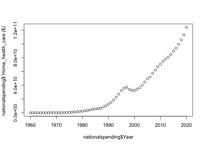
plot(nationalspending$Year, nationalspending$`Home_health_care ($)`)
We can observe from the plot that there is a correlation between Home health care and year. As year increase the spending of home healthcare increase too where it stay constant until 1980 then increase from 1990 to fall a little from 1996 to 2001 and re increase until 2020. this can be explained also demographics. 1996 represents the year of last millennials born which means less expenses on healthcare.
cor(nationalspending$`Home_health_care ($)`, nationalspending$Year)

## [1] 0.9130859
The relationship between home health care and year can be considered positive and strong as the correlation coefficient 0.9130859 turns out to be closer to 1
HH_model <- lm(nationalspending$`Home_health_care ($)` ~ nationalspending$Year)
summary(HH_model)

##
## Call:
## lm(formula = nationalspending$`Home_health_care ($)` ~ nationalspending$Year)
##
## Residuals:
##        Min         1Q     Median         3Q        Max
## -1.786e+10 -1.256e+10 -3.659e+09  1.015e+10  3.986e+10
##
## Coefficients:
##                         Estimate Std. Error t value Pr(>|t|)
## (Intercept)           -3.570e+12  2.093e+11  -17.06   <2e-16 ***
## nationalspending$Year  1.809e+09  1.052e+08   17.20   <2e-16 ***
## ---
## Signif. codes:  0 '***' 0.001 '**' 0.01 '*' 0.05 '.' 0.1 ' ' 1
##
## Residual standard error: 1.446e+10 on 59 degrees of freedom
## Multiple R-squared:  0.8337, Adjusted R-squared:  0.8309
## F-statistic: 295.8 on 1 and 59 DF,  p-value: < 2.2e-16
Both multiple R square and adjusted are > 80 percent , Based on the plot, linear model statistics and correlation coefficient for the relationship between home healthcare and year is evident that the relationship is positive, linear and relatively strong.
Graphical Analysis
plot(nationalspending$Year, nationalspending$`Personal_healthcare ($)`)
 by
looking at this plot we can first see that we have a pretty strong
positive correlation between personal healthcare spending and year
because it keeps increasing from 1960 to 2020and remain constant until
1980 then slightly increase until 1990 to rise again until now. This can
be explains by demographics, technology innovation and increase of
income.
cor(nationalspending$`Personal_healthcare ($)`, nationalspending$Year)

## [1] 0.9399102
The relationship between personal health care and year can be considered positive and strong as the correlation coefficient 0.9399102 turns out to be closer to 1.
PHh_model <- lm(nationalspending$`Personal_healthcare ($)` ~ nationalspending$Year)
summary(PHh_model)

##
## Call:
## lm(formula = nationalspending$`Personal_healthcare ($)` ~ nationalspending$Year)
##
## Residuals:
##        Min         1Q     Median         3Q        Max
## -3.821e+11 -3.400e+11 -7.165e+10  2.355e+11  7.945e+11
##
## Coefficients:
##                         Estimate Std. Error t value Pr(>|t|)
## (Intercept)           -1.044e+14  4.981e+12  -20.95   <2e-16 ***
## nationalspending$Year  5.293e+10  2.503e+09   21.15   <2e-16 ***
## ---
## Signif. codes:  0 '***' 0.001 '**' 0.01 '*' 0.05 '.' 0.1 ' ' 1
##
## Residual standard error: 3.442e+11 on 59 degrees of freedom
## Multiple R-squared:  0.8834, Adjusted R-squared:  0.8815
## F-statistic: 447.1 on 1 and 59 DF,  p-value: < 2.2e-16
Both multiple R square and adjusted are > 80 percent which is pretty close 100% , Based on the plot, linear model statistics and correlation coefficient for the relationship between home healthcare and year is evident that the relationship is positive, linear and relatively strong.
Graphical Analysis
plot(nationalspending$Year, nationalspending$`Out_of_pocket ($)`)
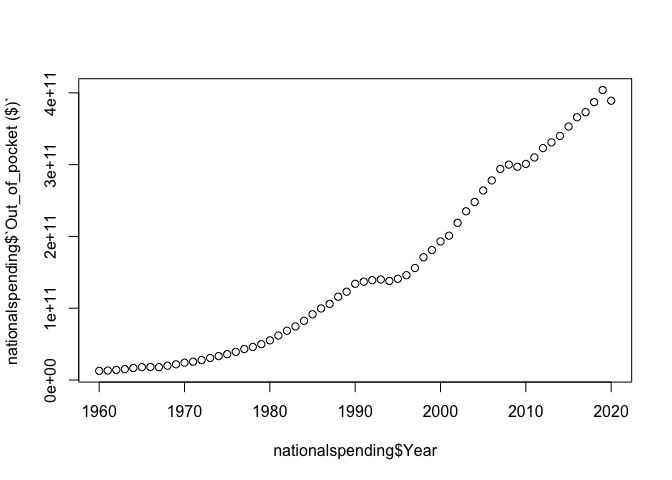 Looking
at the pattern we can that as year increase, expense out of pocket in
health care increase too. we can then affirm that there is a positive
correlation between both variables. Other than that, we observe three
slightly pattern where the out of pocket remain steady then start
increase. from 1960 to 1990 which can be explained by demographic
increase in birth ( millennials), from 2000 to 2010 can explain by the
great recession 2008 then 2010 to 2020 which was affected by both the
recession and recently covid 19.
Testing for correlation between variables
cor(nationalspending$`Out_of_pocket ($)`, nationalspending$Year)

## [1] 0.9701507
The relationship between out of pocket expense and year can be considered positive and strong as the correlation coefficient 0.9701507 turns out to be closer to 1.
Linear regression analysis
OP_model <- lm(nationalspending$`Out_of_pocket ($)` ~ nationalspending$Year)
summary(OP_model)

##
## Call:
## lm(formula = nationalspending$`Out_of_pocket ($)` ~ nationalspending$Year)
##
## Residuals:
##        Min         1Q     Median         3Q        Max
## -4.731e+10 -2.661e+10 -5.470e+09  2.374e+10  6.537e+10
##
## Coefficients:
##                         Estimate Std. Error t value Pr(>|t|)
## (Intercept)           -1.344e+13  4.424e+11  -30.38   <2e-16 ***
## nationalspending$Year  6.830e+09  2.223e+08   30.73   <2e-16 ***
## ---
## Signif. codes:  0 '***' 0.001 '**' 0.01 '*' 0.05 '.' 0.1 ' ' 1
##
## Residual standard error: 3.057e+10 on 59 degrees of freedom
## Multiple R-squared:  0.9412, Adjusted R-squared:  0.9402
## F-statistic: 944.3 on 1 and 59 DF,  p-value: < 2.2e-16
Both multiple R square and adjusted are > 90 percent which is pretty close 100% , Based on the plot, linear model statistics and correlation coefficient for the relationship between Out of pocket expense in healthcare and year is evident that the relationship is positive, linear and relatively strong.
Graphical Analysis
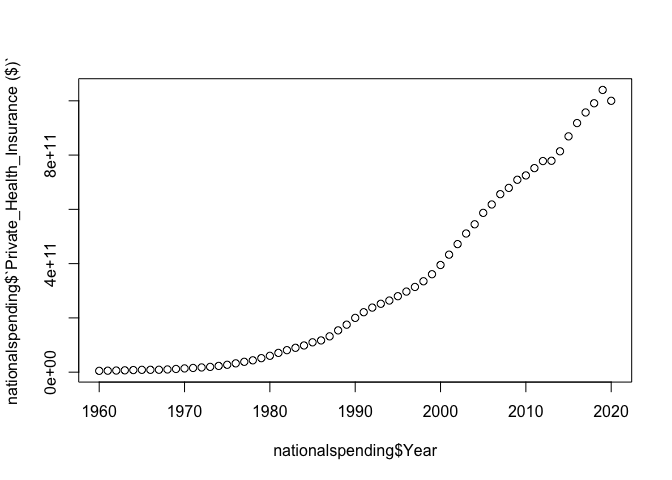
plot(nationalspending$Year, nationalspending$`Private_Health_Insurance ($)`)
At first look we can say that the relationship between private health insurance and year is strong and positive. we can also observe that spending on private kept increasing from 1960 until 2019. This can be explained by demographics and new insurance business because the more population increase the more people are available on the market. The decrease that can observe from 2019 can be explained by covid 19 which has cause many death and also also people were not working so thehy will not be abale to pay their monthly insurance.
Testing for correlation between variables
cor(nationalspending$`Private_Health_Insurance ($)`, nationalspending$Year)

## [1] 0.9432591
With a correlation of 0.9432591, we can say there is strong positive relationship between Private insurance and year.
Linear regression analysis
PH_model <- lm(nationalspending$`Private_Health_Insurance ($)` ~ nationalspending$Year)
summary(PH_model)

##
## Call:
## lm(formula = nationalspending$`Private_Health_Insurance ($)` ~
##     nationalspending$Year)
##
## Residuals:
##        Min         1Q     Median         3Q        Max
## -1.341e+11 -1.152e+11 -1.543e+10  7.495e+10  2.134e+11
##
## Coefficients:
##                         Estimate Std. Error t value Pr(>|t|)
## (Intercept)           -3.454e+13  1.598e+12  -21.62   <2e-16 ***
## nationalspending$Year  1.752e+10  8.027e+08   21.82   <2e-16 ***
## ---
## Signif. codes:  0 '***' 0.001 '**' 0.01 '*' 0.05 '.' 0.1 ' ' 1
##
## Residual standard error: 1.104e+11 on 59 degrees of freedom
## Multiple R-squared:  0.8897, Adjusted R-squared:  0.8879
## F-statistic: 476.1 on 1 and 59 DF,  p-value: < 2.2e-16
Both multiple R square and adjusted are > 80 percent which is pretty close 100% , Based on the plot, linear model statistics and correlation coefficient for the relationship between private health insurance and year is evident that the relationship is positive, linear and relatively strong.
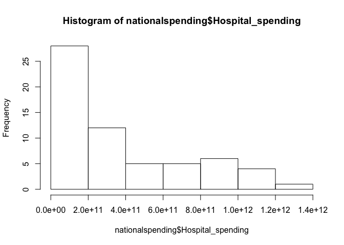
hist( x = nationalspending$Hospital_spending)
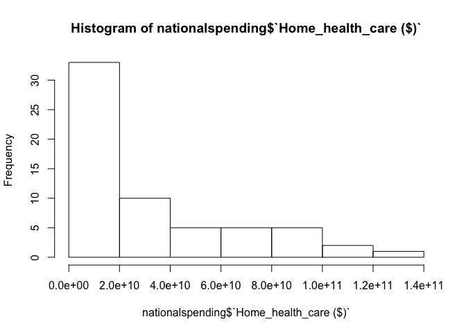
hist( x = nationalspending$`Home_health_care ($)`)
hist( x = nationalspending$`Personal_healthcare ($)`)
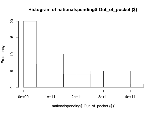
hist( x = nationalspending$`Out_of_pocket ($)`)
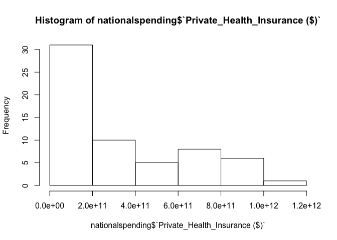
hist( x = nationalspending$`Private_Health_Insurance ($)`)
HS <- sum(nationalspending$Hospital_spending)
HH <- sum(nationalspending$`Home_health_care ($)`)
PHC <- sum(nationalspending$`Personal_healthcare ($)`)
OP <- sum(nationalspending$`Out_of_pocket ($)`)
PH <- sum(nationalspending$`Private_Health_Insurance ($)`)

Slices <- c("HS","HH","PHC","OP","PH")
lbls <- c("Hospitalspending", "homehealthcare", "personalhealthcare", "Outofpocket", "privatehealthins")
R Markdown is a file format that help you turn your analysis in high quality documents, reports, presentations and dashboard. During the beginning of the semester, we have learned how to use R markdown through class and the assignments. I created a new R Markdown that I am using for this project. it will help make my finding clean and neat in readable pdf documents. I will know my R markdown file once I am done into a pdf format.
- Using the steps from homework 1, 2,3 to examine data ## Analyzing data by creating Histogram and plot ## Data Cleaning
During class, which I utilized to turn in the draft of this final project. I created a new repository on Github, copied the link, pasted it into a new project on R, then committed it, and lastly pushed the commit to Github using an authentication token. I have minimal experience with Git, so I followed the instructions on Canvas. In the past, I learned how to use Git with Terminal, but using it with R is new to me. In the past, I pushed projects to Git through terminal commands. Although we did not spend much time with Github during this semester, I plan to explore it further outside of class.
Linear regression is commonly used type of predictive analysis. It is a statistical approach for modeling the relationship between a dependent variable and a given set of independent variables. In our case, we will used the simple linear regression because we want to summarize and study the relationships between two variables. During class, We have learned how to use to conduct our analysis. I have created a model for each category spending and year to test if there was a relationship. To do so, I have tested the correlation first then plotting to see if visualize it. I have to admit that working with liner regression was a bit difficult but going back to lecture and notes help me to run the model and analyze it.
Although pie charts are not really recommended in R, I wanted to give a visual representation of all spending in histogram and pie so that the reader can have an visual idea of much was spent on each spending category all this year. I could not make the code for the pie since it was not working for me. here the I tried to use
Slices <- c(“HS”,“HH”,“PHC”,“OP”,“PH”) lbls <- c(“Hospitalspending”, “homehealthcare”, “personalhealthcare”, “Outofpocket”, “privatehealthins”)
pie(“Slices”, “labels” = lbls, main=“National_spending on healthcare”)
after testing all the models ( HH_model, HS_model, PH!_model, OP_model and PH_model ) we can affirm that each spending category increase as year increase too. this is due to many factors such as economics, demographics, pandemic and many others. As for determining if the spending will continue to increase or not. We can not confidently affirm that we will increase or not. However, when looking at different plot we see that the trend continue to incline in hospital spending, home health care , personal insurance and started to decline in out of pocket healthcare, private insurance. TO be more confident about predicting it, we will need to run more analysis which was my goal but As I was trying other analysis method such Polynomial regression or ridge regression I could not really get any result. Overall, I can confidently say have more some progress using R studio. At the beginnings of this class I was completely new to it and had no idea if I was going to even able to do this on my own but the homework, lecture and research definitely gave a footsteps in R and I am even eager to learn more and more codes to be able to apply my knowledge in a workplace. This is definitely a millstone in R studio journey.
https://www.upgrad.com/blog/types-of-regression-models-in-machine-learning/#:~:text=Linear%20regression%20and%20logistic%20regression,most%20prominent%20techniques%20of%20regression. https://www.statology.org/correlation-vs-association/ https://www.geeksforgeeks.org/create-multiple-pie-charts-using-ggplot2-in-r/?ref=rp https://www.usatoday.com/story/money/2020/09/06/the-worlds-most-important-event-every-year-since-1920/113604790/
