"Momentum" in optimization theory is usually introduced as an ad-hoc improvement over vanilla gradient descent. By leveraging moving averages over gradients, the optimizer manages not to get stuck in inflections or bad minimas. But momentum is so much more. Quoted from this brilliant article:
"For now — momentum is an algorithm for the book."
Reference: ME697 Advanced Scientific Machine Learning
Forget all about optimization and gradient descent for now and focus on basic mechanics.
If a object lies in a potential energy field, it experiences a force. The force acting at any point
Consider two worlds:
- Sticky World: The velocity of the object is proportional to the net force.
- Newton's World: The acceleration of the object is proportional to the net force.
We imagine these world's in 1D and visualize them in 2D. On the X axis you have the position of the object. On Y axis you have the potential energy.
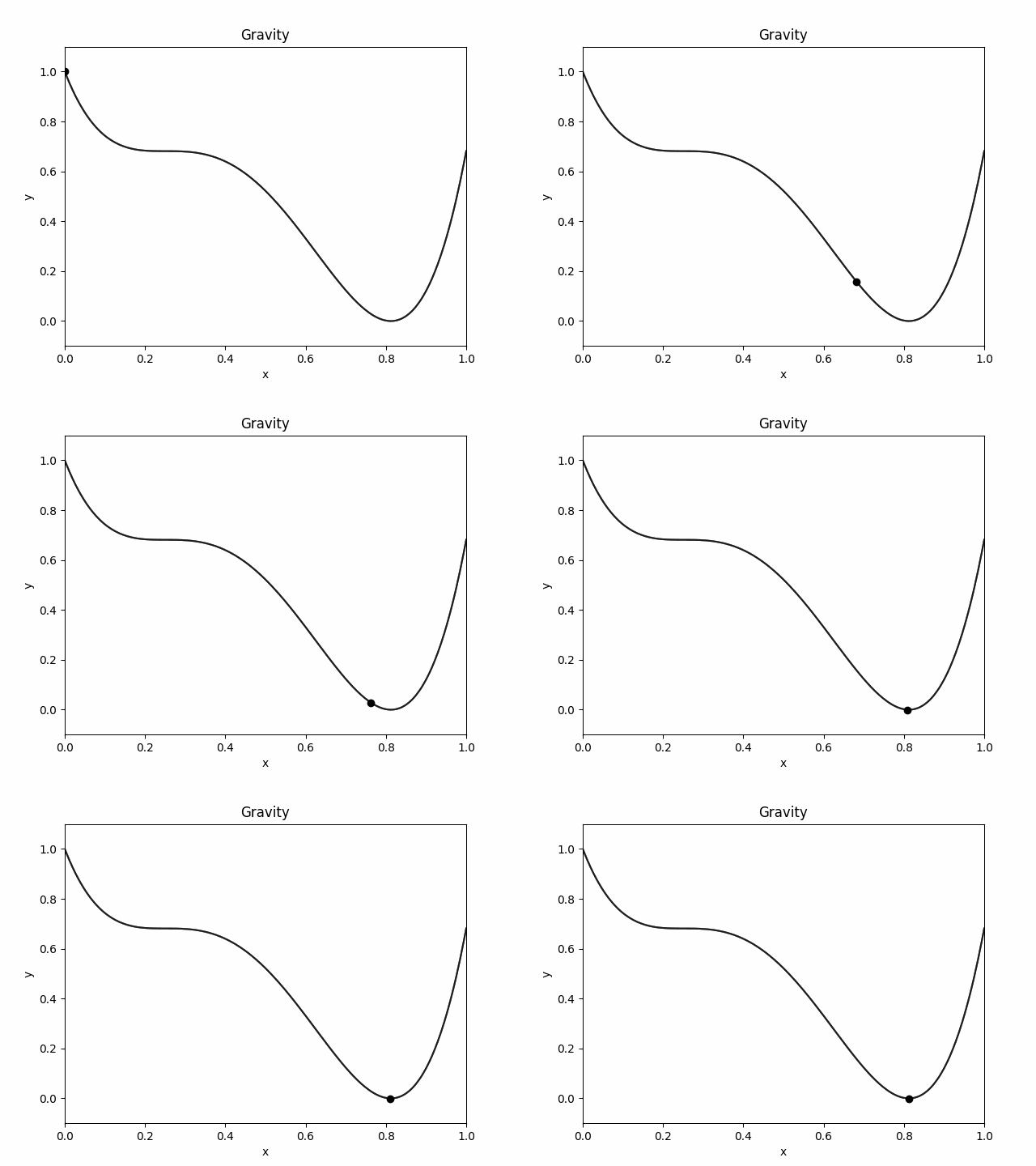
Here is how the object moves in `Sticky World':

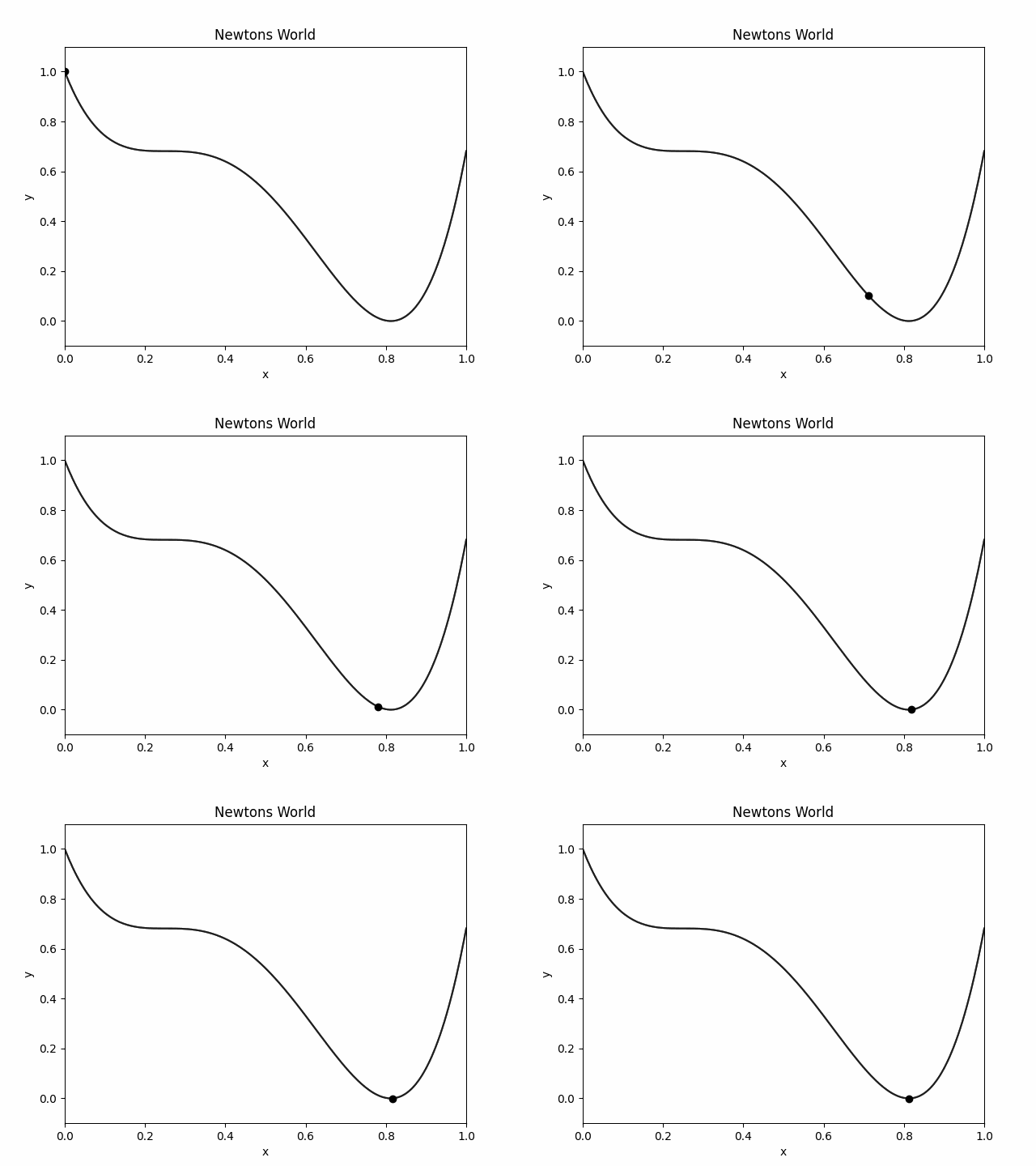
Here is how the object moves in `Newton's World':
 Note: We have also employed a drag force here, acting in direction opposing the momentum, proportional to it.
Observations:
- There is no inertia in the sticky world. Any maxima, minima or inflection (
$\nabla_x f(x) = 0$ ) makes the velocity/momentum of the object zero. The object stops. - In newton's world, there is inertia. When force is zero, the object stops accelerating but it still moves.
- Newton's world has better chances of a object not getting stuck in shallows and inflections.
Conclusions:
- The sticky world is a direct analogy to gradient descent:
$$m\dot{x} \propto -\nabla_x f$$ $$\dot{x} \propto -\nabla_x f$$ $$\lim_{{\delta t} \to 0} \frac{x_{t+\delta t} - x_t}{\delta t} \propto -\nabla_x f$$
Considering a discrete equivalent case:
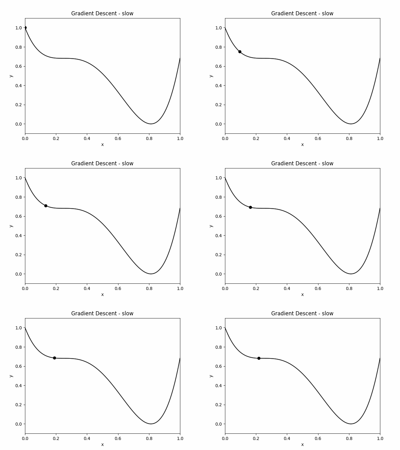
Let's just implement gradient descent on the potential energy function.
Doesn't this look identical to sticky world? It is important to note that these are two completely different solvers. The sticky world simulation was made by solving a ODE of a bead on a wire. This is just a iterative optimization animation.
2. Newton's world is an analogy to gradient descent with momentum:
This can be converted into a ODE, by chosing another variable
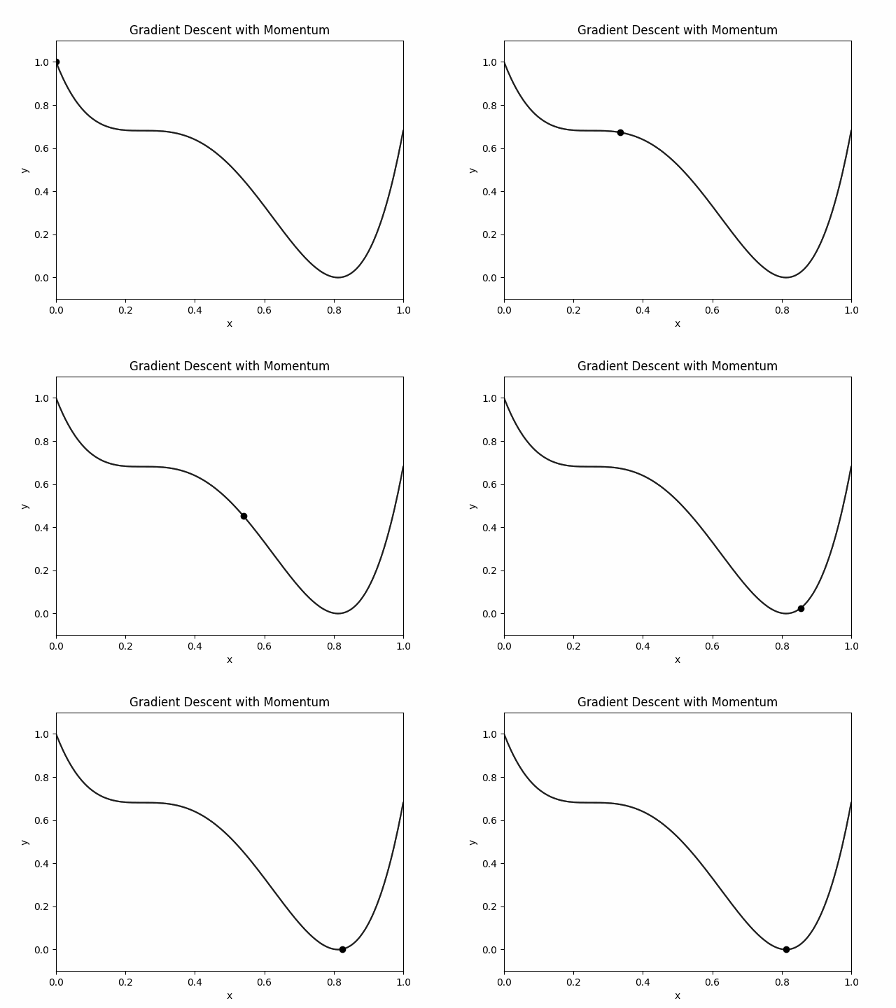
This is gradient descent with momentum!
Doesn't this look identical to newtons world? Again, note that these are two completely different solvers.
Visualizing optimization as a mechanics problem led to a better algorithm.
Incomplete
For now, consider a body of mass
Consider two forces,
This is a pretty general mechanics problem statement - A free moving body operating under a force induced by a potential energy field and some friction. Consier, a 1-D space where each point
Now for the hard part. You may have often tried to visualize a higher dimensional space in a lower dimension. I am going to ask you to do the opposite. Imagine this 1-D space in 2-D. The first dimension
You can think of the body as a bead on a wire. The shape of the wire is
(YET to complete)


