In this post, I’ll use simulation and optimization to determine which draft strategies will result in the best lineups for fantasy football.
In fantasy football, there’s a lot to consider when trying to figure out an optimal draft strategy. Top RB’s have a high ceiling and the potential to score 350 points, whereas top WRs can only reach 275 points, however top WR’s are usually seen as safer as they have a higher correlation of their preseason to end of season rank. Positions like DST, which have low ceiling and low pre-season correlation seem to be an obvious choice to draft very late. There’s a lot of things to consider, and I haven’t even mentioned other things like how you need to start a different number of each position. Simulation is a good way to estimate the effects of different strategies.
The first thing I’ll do is organize/plot the data. I’m using season projections from FantasyData.com, fantasyfootballanalytics.net, and FFToday.com because they have archived projections available. I’m using Average Draft Position (ADP) data from fantasyfootballcalculator.com which shows where players were drafted each year. For all of this, I’m using Half-PPR scoring and Yahoo defaults (1 QB, 2 RB, 2 WR, 1 TE, 1 RB/WR/TE, 1 DST, 1K). To start off I’ll look at some summary stats:
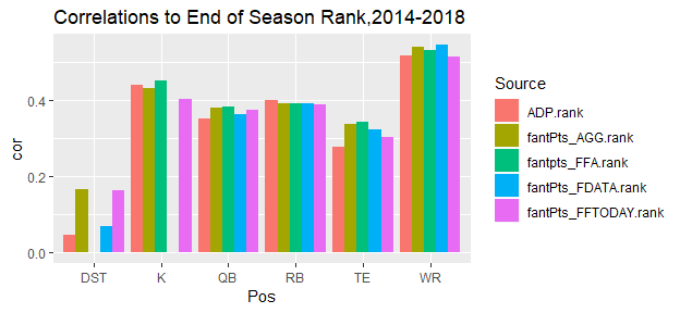
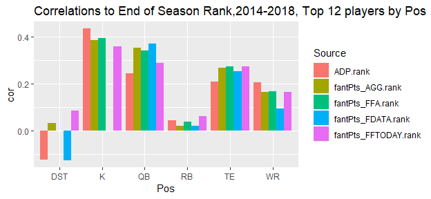
From this chart, you can see that certain positions are easier to project. DST expectedly is very hard to rank preseason so is an obvious candidate to draft late. You can also see that the outside ranks have similar predictive accuracy to ADP.Rank. AGG.rank is just the mean of the outside ranks. This plot is a bit unfair though, because positions with a larger sample size will have their correlation unfairly inflated due to being able to rank further down into benchwarmer players. I’ll reproduce the plot with the top 12 for each position:
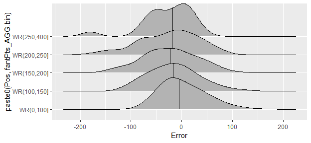
In addition, I’d also like to summarize the errors/variance:
Above I show the distribution of errors for WRs, from 2008-2018. I am going to use this when I make my draft strategy. I want to know based on the projection and the Pos, how the error is distributed. Positive error means they overperformed their projection. Now that the data is prepared and summarized, I’m ready to test out a system.
After preparing the data and organizing estimated projections and errors, I’m ready to test out draft strategies. I want something like this, which shows how a different strategy in R1-3 will affect a draft’s projected points. This is meant to let you see what positions you should wait on drafting if you want to maximize your points. The thing that isn’t accounted for in the above link though, is that in reality you are not trying to maximize projected points of a full draft, but rather for your eventual starting lineup, so you’re trying to pick the draft that will give you the best eventual nine players.
My methodology consists of two functions: getPicks() and simSeason().
getPicks() takes in parameters like the slot you are drafting at, numRBs to draft, numWR to draft, and you can fix/exclude players or positions for each round as well. It then returns the draft which maximizes total points of all the picks, given the specified parameters and draft-position constraints. I show an example below, maximizing the points for Slot7/12 in a 15 round draft.
picks<-getPicks(slot="Slot7", data=all.data[all.data$Season==2019,], numTeams = 12,
                numRB=4, numWR = 5,numTE=2,numQB=2,numK=1, numDST=1)
## Player Pos Team ADP_half ADP.Rank fantPts_AGG fantPts_AGG.bin Slot
## 10727 Julio Jones WR Atl 11.0 11.0 260.6014 (250,400] 7
## 10734 Todd Gurley RB Lar 17.0 18.0 230.9717 (200,250] 18
## 10752 George Kittle TE Sfo 33.3 36.0 193.4550 (150,200] 31
## 10759 Phillip Lindsay RB Den 42.6 43.0 193.0022 (150,200] 42
## 10779 James White RB Nwe 62.2 63.0 173.3381 (150,200] 55
## 10789 Alshon Jeffery WR Phi 71.7 73.0 169.2632 (150,200] 66
## 10798 Allen Robinson WR Chi 80.0 82.0 157.8520 (150,200] 79
## 10824 Corey Davis WR Ten 105.9 108.0 153.1803 (150,200] 90
## 10827 Lesean Mccoy RB Buf 108.2 110.5 146.5663 (100,150] 103
## 10830 Jameis Winston QB Tam 111.8 114.0 297.6446 (250,400] 114
## 10845 Bal DST Bal 124.6 129.0 110.0000 (100,150] 127
## 10854 Dak Prescott QB Dal 131.9 138.0 296.9355 (250,400] 138
## 10867 Greg Zuerlein K Lar 147.2 151.5 123.1068 (100,150] 151
## 10890 Kyle Rudolph TE Min 159.6 174.0 118.2575 (100,150] 162
## 11107 Mohamed Sanu WR Atl NA 500.0 131.2559 (100,150] 175
Above I display the optimal planned-draft given my parameters. You can
see how each player’s ADP.Rank must be greater than or equal to the slot
they are drafted at.
The second function is simSeason() which takes in the above planned-draft from getPicks(), and using the errors from earlier, samples from the errors in the player’s corresponding position/projection-bin to get a simulated score. Using this, I can then sort by simulated score to get the starting lineup from my draft. You only can put 9 players in your starting lineup and so if you have 2 amazing QBs in the simulated scores, only 1 will get into your simulated starting lineup. In addition, I also simulate the scores of the undrafted players, and I assume you are able to add the 4th-best simulated undrafted player at each position. I made this assumption because it is likely you will be lacking at 1-2 positions and so will be able to get a decent player as a pickup for those positions.
Below you can see an example using the above picks:
set.seed(1)
topLineup<-simSeason(picks = picks, data=all.data, numSims=1,
                     numRB = 2, numWR=2, numFLEX = 1,  numQB=1, numTE = 1, numDST = 1, numK = 1   )
## Player Pos Team ADP_half ADP.Rank fantPts_AGG fantPts_AGG.bin Slot error Sim Pickup
## 12 Dak Prescott QB Dal 131.9 138.0 296.9355 (250,400] 138 -5.942500 290.9930 0
## 1 Julio Jones WR Atl 11.0 11.0 260.6014 (250,400] 7 19.683333 280.2847 0
## 8 Corey Davis WR Ten 105.9 108.0 153.1803 (150,200] 90 106.528507 259.7088 0
## 4 Phillip Lindsay RB Den 42.6 43.0 193.0022 (150,200] 42 7.255476 200.2577 0
## 3 George Kittle TE Sfo 33.3 36.0 193.4550 (150,200] 31 3.537667 196.9927 0
## 9 Lesean Mccoy RB Buf 108.2 110.5 146.5663 (100,150] 103 2.115981 148.6822 0
## 13 Greg Zuerlein K Lar 147.2 151.5 123.1068 (100,150] 151 16.114583 139.2214 0
## 18 Chris Hogan WR Car NA 500.0 65.1050 (0,100] NA 66.172444 131.2774 1
## 20 Nyg DST Nyg NA 500.0 81.0000 (0,100] NA 27.000000 108.0000 1
You can see from “error”, which players over and underperformed in the sim, sampling the error from 2008-2018 data. Additionally, in the above sim you see how a player can make it into the top starting lineup as a pickup if their simmed score was better than a drafted player. I can now repeat simseason() many times, and so can get a mean simulated-lineup-total-score for the planned picks. I used 2000 as my simulation size as it seemed sufficient for the mean to converge.
topLineups<-simSeason(picks = picks, data=all.data, numSims=2000,
                      numRB = 2, numWR=2, numFLEX = 1,
                      numQB=1, numTE = 1, numDST = 1, numK = 1   )
summary(sapply(topLineups, function(x) sum(x$Sim)))
## Min. 1st Qu. Median Mean 3rd Qu. Max.
## 1363 1638 1729 1732 1821 2171
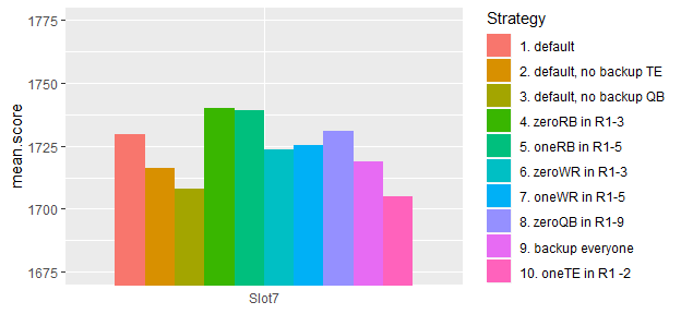
Now I’m ready to test different getPicks() parameters to see how I should do my draft to get my the best mean-starting lineup. I included arguments in the getPicks() function such as onePos and outPos which can allow me to force positions in/out of rounds and experiment with strategies like “have exactly one TE in Rounds 1-2” or “exactly zero RB in Rounds 1-4”, or other things. I test out several parameter combinations below for the 7th slot of a 12 team, 15 round draft.
And there are the detailed parameters with each strategy:
##    Strategy.ID numRB numWR numTE numQB numK numDST  Constraints.Comments
## 1            1     4     5     2     2    1      1               default
## 2            2     5     5     1     2    1      1 default, no backup TE
## 3            3     5     5     2     1    1      1 default, no backup QB
## 4            4     5     4     2     2    1      1        zeroRB in R1-3
## 5            5     5     4     2     2    1      1         oneRB in R1-5
## 6            6     4     5     2     2    1      1        zeroWR in R1-3
## 7            7     4     5     2     2    1      1         oneWR in R1-5
## 8            8     4     5     2     2    1      1        zeroQB in R1-9
## 9            9     3     4     2     2    2      2       backup everyone
## 10          10     4     5     2     2    1      1        oneTE in R1 -2
Based on the above, you can see how certain strategies don’t really make a difference, and certain ones perform worse. For example the zero-WR strategy (6) performs worse than the zero-RB strategy. Not taking a backup TE and QB also worsen the score.
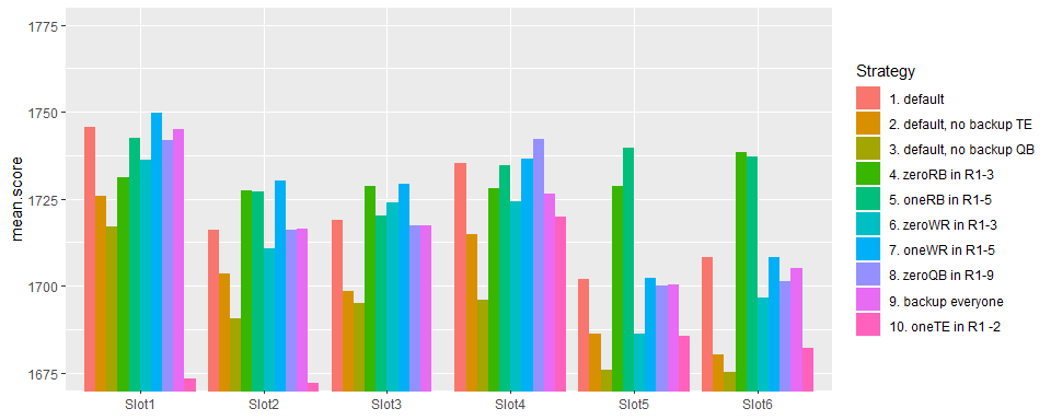
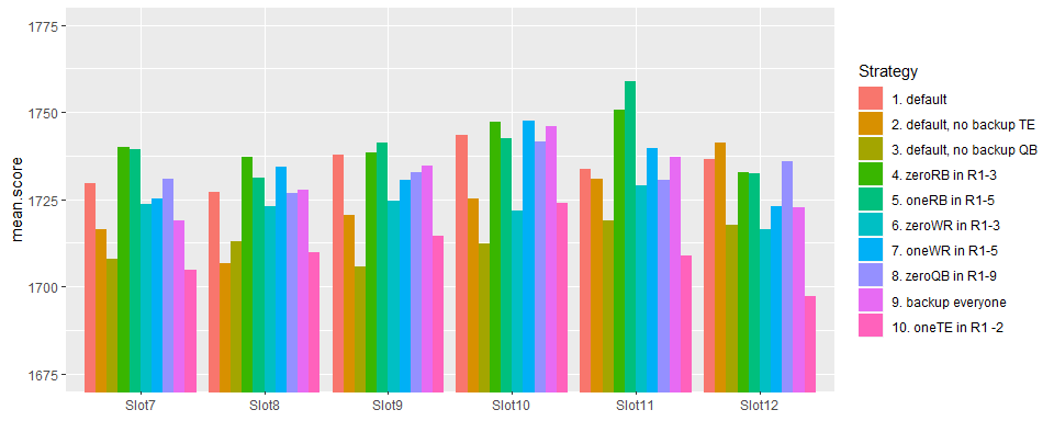
Finally, I reproduce this for all draft slots. Below you can see the results, and how the best strategy is affected by your draft slot.
In the above plots you can see strategy performance for each draft slot. For many of the slots the chosen strategy actually does not seem to have a huge effect, which is interesting. Some things do make a difference though--not taking a backup QB (strategy 3) seems to have a large negative effect for all draft positions. Not taking a backup TE (#2) also appears to have a negative impact. I guess the waiver adds you can get for these positions are not as good as someone you can get through the draft. In addition, for many of the slots doing zero-RB (4&5) seems to be better than zero-WR (6&7).
This is just for Half-PPR 12 man leagues, and the results might change with different scoring but it at least is an attempt to quantitatively evaluate strategies.
Looking at the strategies, many of them perform similarly, finishing within 10-20 points. Zero RB does seem to preform better than zero WR, but in general, strategy seems to have only a small effect for most of the draft slots. If a league requires 3 WRs to start then this will probably favor an early WR strategy further, and if the scoring is PPR or STD then that might have an effect too. Parameter changes like taking a backup QB seemed to have a large effect accross the board.
Another takeaway is that projections have been about as accurate as ADP. I wouldn’t just go by a projection model or trust someone until I’ve seen it is proven to be useful, even if they try to make it sound complex. WRs do appear to be somewhat easier to outperform ADP and so I think it makes sense to work on a model for them or find someone who has an accurate one.
Finally, there are a couple shortcomings with my method. Firstly, I am not accounting for opponent probabilistic picking i.e. the fact that you don’t know exactly where a player will be picked. For simplicity I left this out. I think estimating a single draft like I did at least shows you things like the effect of going RB early and WR late, and keeps it simpler, despite the available players not being exact. Accounting for this though would be complicated as I’d have to return a set of potential drafts with getPicks() instead of a single draft, so I wanted to keep it simple for now. Comparing the results of a probabalistic pick system to the current system would be a useful project.
The second main shortcoming I think is that the optimal strategy determined by the system will be dependent on the projections I supply. For example, if there is a WR that is projected as hugely undervalued in the 10th round, then doing a WR-early, RB-late strategy will look bad because I am missing out on that value. I think this is something I should look into. Having said that, things like taking a backup QB/TE seem like they’d be less affected by this. An interesting idea would be to create an entirely ADP-based projection model so that I can see how the optimal strategy would be regardless of projection system i.e. if there are no sleepers.
TLDR: Most strategies did similarly. It does seem that you should definitely take a backup QB, and also a backup TE especially if you don’t take a TE early. Other than that I haven’t found any shocking secrets yet that will give me a huge edge. Thanks for reading!
