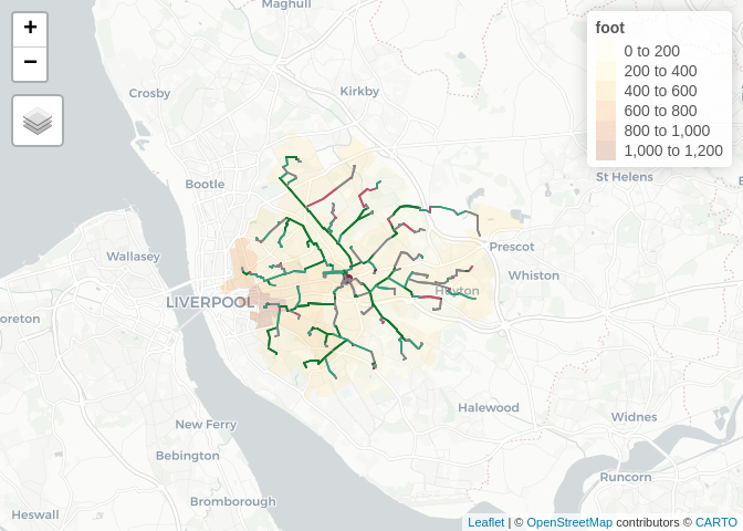
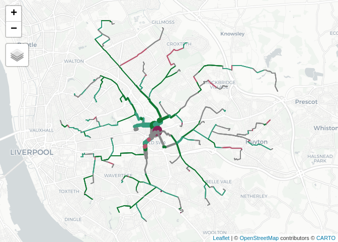
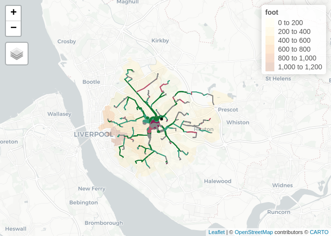
The aim of this document is to demonstrate how to convert Origin-Destination data to route networks. The data for this is from the wicid website.
You can download datasets at multiple geographic levels from that website. We will start with the open MSOA to MSOA dataset.
The study location can be defined as follows:
study_location_name = "Alder Hey Children's Hospital"
study_location_coodinates = tmaptools::geocode_OSM(study_location_name)$coords
study_location_coodinates
x y
-2.896989 53.419608
study_location_df = data.frame(name = study_location_name, lon = study_location_coodinates[1], lat = study_location_coodinates[2])
study_location_sf = sf::st_as_sf(study_location_df, coords = c("lon", "lat"), crs = 4326)
buffer_distance = 5000
study_location_buffer = sf::st_buffer(study_location_sf, buffer_distance)
For the MSOA data we will get data from the pct R package as follows:
msoa_data = pct::get_pct(layer = "z", geography = "msoa", national = TRUE)We will also get population weighted centroids for the MSOA data:
msoa_centroids = pct::get_pct(layer = "c", geography = "msoa", national = TRUE)Let’s find the administrative zones the centroids of which are within the buffer:
centroids_msoa = msoa_centroids[study_location_buffer, ]
zones_msoa = msoa_data |>
  filter(geo_code %in% centroids_msoa$geo_code)
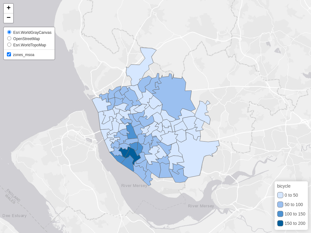
We can visualise the results as follows:
m = tm_shape(zones_msoa) +
  tm_polygons("bicycle")
tmap_save(m, "msoa_zones.html")
browseURL("msoa_zones.html")
Let’s subset the data that originates in the study location and which goes the the MSOA within which the study location is located:
zone_study_area = zones_msoa[study_location_sf, ]
u_od_msoa = "https://s3-eu-west-1.amazonaws.com/statistics.digitalresources.jisc.ac.uk/dkan/files/FLOW/wu03ew_v2/wu03ew_v2.zip"
f_od_msoa = basename(u_od_msoa)
if(!file.exists(f_od_msoa)) {
  download.file(u_od_msoa, f_od_msoa)
  unzip(f_od_msoa)
}
od_all = read_csv("wu03ew_v2.csv")
od_msoa = od_all |>
  filter(`Area of residence` %in% zones_msoa$geo_code) |>
  filter(`Area of workplace` %in% zone_study_area$geo_code)
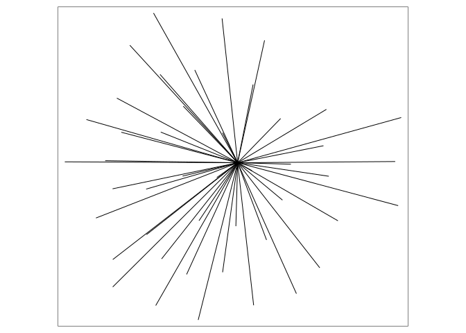
We can plot the resulting OD data as follows:
od_msoa$`Area of workplace` = study_location_sf$name
desire_lines = od::od_to_sf(od_msoa, zones_msoa, zd = study_location_sf)
tm_shape(desire_lines) +
  tm_lines()
We’ll save the MSOA data as follows:
write_csv(od_msoa, "od_msoa.csv")
sf::write_sf(zones_msoa, "zones_msoa.geojson", delete_dsn = TRUE)
sf::write_sf(desire_lines, "desire_lines.geojson", delete_dsn = TRUE)
sf::write_sf(centroids_msoa, "centroids_msoa.geojson", delete_dsn = TRUE)
sf::write_sf(study_location_buffer, "study_location_buffer.geojson", delete_dsn = TRUE)
sf::write_sf(study_location_sf, "study_location.geojson", delete_dsn = TRUE)
Let’s calculate routes for each OD pair:
routes_msoa = stplanr::route(l = desire_lines, route_fun = cyclestreets::journey, plan = "quietest")
sf::write_sf(routes_msoa, "routes_msoa.geojson", delete_dsn = TRUE)
We’ll read-in the pre-saved routes as follows.
routes_msoa = sf::read_sf("routes_msoa.geojson")names(routes_msoa) [1] "Area of residence"
[2] "Area of workplace"
[3] "All categories: Method of travel to work"
[4] "Work mainly at or from home"
[5] "Underground, metro, light rail, tram"
[6] "Train"
[7] "Bus, minibus or coach"
[8] "Taxi"
[9] "Motorcycle, scooter or moped"
[10] "Driving a car or van"
[11] "Passenger in a car or van"
[12] "Bicycle"
[13] "On foot"
[14] "Other method of travel to work"
[15] "route_number"
[16] "id"
[17] "time"
[18] "busynance"
[19] "quietness"
[20] "signalledJunctions"
[21] "signalledCrossings"
[22] "name"
[23] "walk"
[24] "elevations"
[25] "distances"
[26] "type"
[27] "legNumber"
[28] "distance"
[29] "turn"
[30] "startBearing"
[31] "color"
[32] "provisionName"
[33] "start"
[34] "finish"
[35] "start_longitude"
[36] "start_latitude"
[37] "finish_longitude"
[38] "finish_latitude"
[39] "crow_fly_distance"
[40] "event"
[41] "whence"
[42] "speed"
[43] "itinerary"
[44] "plan"
[45] "note"
[46] "length"
[47] "west"
[48] "south"
[49] "east"
[50] "north"
[51] "leaving"
[52] "arriving"
[53] "grammesCO2saved"
[54] "calories"
[55] "edition"
[56] "gradient_segment"
[57] "elevation_change"
[58] "gradient_smooth"
[59] "geometry"
library(sf)
attrib = c("Bicycle", "On foot", "gradient_smooth", "quietness", "All categories: Method of travel to work")
routes_msoa_minimal = routes_msoa[, attrib] |>
  mutate(quietness = as.numeric(quietness))
rnet_msoa_raw = stplanr::overline(routes_msoa_minimal, attrib = attrib, fun = list(sum = sum, mean = mean))
rnet_msoa_quiet = rnet_msoa_raw |>
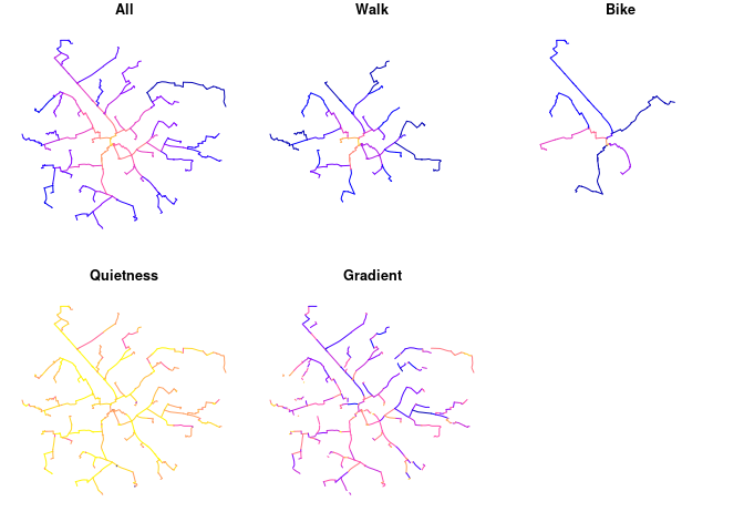
  transmute(All = `All categories: Method of travel to work_sum`, Walk = `On foot_sum`, Bike = Bicycle_sum, Quietness = quietness_mean, Gradient = gradient_smooth_mean)
sf::write_sf(rnet_msoa_quiet, "rnet_msoa_quiet.geojson", delete_dsn = TRUE)
plot(rnet_msoa_quiet, logz = TRUE)
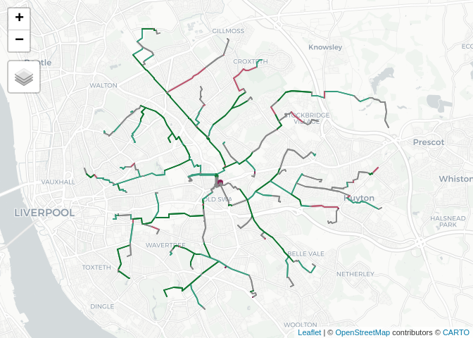
We’ll create an interactive map of the outputs as follows, building on the CRUSE project:
remotes::install_github("ITSLeeds/netvis")
basemaps = c(
  `Grey basemap` = "CartoDB.Positron",
  `Coloured basemap` = "Esri.WorldTopoMap"
  # `Cycleways (OSM)` = "https://b.tile-cyclosm.openstreetmap.fr/cyclosm/{z}/{x}/{y}.png",
  # `Satellite image` = "https://server.arcgisonline.com/ArcGIS/rest/services/World_Imagery/MapServer/tile/{z}/{y}/{x}'"
)
popup_vars = c(
  "Cycle friendliness" = "Quietness",
  "Gradient" = "Gradient"
)
quietness_palette = pal = c('#882255','#CC6677', '#44AA99', '#117733')
map_rnet = netvis::netvis(
  rnet_msoa_quiet,
  width_regex = "Bik|Walk",
  popup_vars = popup_vars,
  width_var_name = "Bicycle trips",
  col = "Quietness",
  pal = pal,
  basemaps = basemaps,
  legend.col.show = FALSE,
  output = "tmap"
  )
tmap_mode("view")
map_rnet
m_combined = tm_shape(zones_msoa, name = "Zones (MSOA)") +
tm_fill("foot", alpha = 0.2) +
map_rnet
m_combinedtmap_save(m_combined, "m_combined_cyclestreets.html")We can calculate uptake as follows.
summary(routes_msoa$distances) Min. 1st Qu. Median Mean 3rd Qu. Max.
1.0 17.0 50.0 154.6 171.0 1828.0
routes_msoa_uptake = routes_msoa |>
  mutate(quietness = as.numeric(quietness)) |>
  group_by(`Area of residence`, `Area of workplace`) |>
  mutate(distance = sum(distances), gradient = weighted.mean(gradient_smooth * distances)) |>
  mutate(pcycle_dutch = pct::uptake_pct_godutch_2020(distance = distance, gradient = gradient)) |>
  mutate(`Bicycle (Go Dutch)` = `All categories: Method of travel to work` * pcycle_dutch)
attrib = c("Bicycle", "Bicycle (Go Dutch)", "On foot", "gradient_smooth", "quietness")
routes_msoa_minimal = routes_msoa_uptake[attrib]
rnet_msoa_raw = stplanr::overline(routes_msoa_uptake, attrib = attrib, fun = list(sum = sum, mean = mean))
rnet_msoa_quiet = rnet_msoa_raw |>
transmute(Walk = `On foot_sum`, Bike = Bicycle_sum, `Bike (Go Dutch)` = round(`Bicycle (Go Dutch)_sum`), Quietness = quietness_mean, Gradient = gradient_smooth_mean)
sf::write_sf(rnet_msoa_quiet, "rnet_msoa_quiet_go_dutch.geojson", delete_dsn = TRUE)We’ll create an interactive map of the outputs as follows, building on the CRUSE project:
popup_vars = c(
  "Cycle friendliness" = "Quietness",
  "Gradient" = "Gradient"
)
quietness_palette = pal = c('#882255','#CC6677', '#44AA99', '#117733')
map_rnet = netvis::netvis(max_width = 19,
  rnet_msoa_quiet,
  width_regex = "Bik|Walk|Go",
  popup_vars = popup_vars,
  width_var_name = "Bicycle trips",
  col = "Quietness",
  pal = pal,
  basemaps = basemaps,
  legend.col.show = FALSE,
  output = "tmap"
  )
tmap_mode("view")
map_rnet
m_combined = tm_shape(zones_msoa, name = "Zones (MSOA)") +
tm_fill("foot", alpha = 0.2) +
map_rnet +
qtm(study_location_sf)
m_combinedtmap_save(m_combined, "m_combined_go_dutch.html")