library(tidyverse)
library(sf)
remotes::install_dev("stats19")
library(stats19)
Data was obtained from the DfT’s STATS19 data releases using the
stats19 R package. The data is available for download from the DfT
website. The
data is available in two forms: as a single file for each year, and as a
single file for each type of data (e.g. collisions, casualties,
vehicles) for all years. The latter is more convenient for analysis, but
the former is more convenient for downloading. The stats19 package
provides functions to download the data in both forms.
The last 5 years of data for the ‘collisions’ and ‘casualties’ tables were downloaded in the first instance. They have the following column names:
collisions = get_stats19("collision", year = "5-years")
casualties = get_stats19("casualty", year = "5-years")
names(collisions)
[1] "accident_index"
[2] "accident_year"
[3] "accident_reference"
[4] "location_easting_osgr"
[5] "location_northing_osgr"
[6] "longitude"
[7] "latitude"
[8] "police_force"
[9] "accident_severity"
[10] "number_of_vehicles"
[11] "number_of_casualties"
[12] "date"
[13] "day_of_week"
[14] "time"
[15] "local_authority_district"
[16] "local_authority_ons_district"
[17] "local_authority_highway"
[18] "first_road_class"
[19] "first_road_number"
[20] "road_type"
[21] "speed_limit"
[22] "junction_detail"
[23] "junction_control"
[24] "second_road_class"
[25] "second_road_number"
[26] "pedestrian_crossing_human_control"
[27] "pedestrian_crossing_physical_facilities"
[28] "light_conditions"
[29] "weather_conditions"
[30] "road_surface_conditions"
[31] "special_conditions_at_site"
[32] "carriageway_hazards"
[33] "urban_or_rural_area"
[34] "did_police_officer_attend_scene_of_accident"
[35] "trunk_road_flag"
[36] "lsoa_of_accident_location"
[37] "datetime"
names(casualties) [1] "accident_index" "accident_year"
[3] "accident_reference" "vehicle_reference"
[5] "casualty_reference" "casualty_class"
[7] "sex_of_casualty" "age_of_casualty"
[9] "age_band_of_casualty" "casualty_severity"
[11] "pedestrian_location" "pedestrian_movement"
[13] "car_passenger" "bus_or_coach_passenger"
[15] "pedestrian_road_maintenance_worker" "casualty_type"
[17] "casualty_home_area_type" "casualty_imd_decile"
[19] "lsoa_of_casualty"
We’ll join the casualties and collisions tables together, and then filter to only include pedestrian and cycling casualties.
cas_types = casualties %>%
  select(accident_index, casualty_type, casualty_severity) %>%
  mutate(n = 1) %>%
  group_by(accident_index, casualty_type, casualty_severity) %>%
  summarise(n = sum(n)) %>%
  tidyr::spread(casualty_type, n, fill = 0)
cas_joined = left_join(collisions, cas_types, by = "accident_index")
Let’s plot the result:
crashes_dates = cas_joined %>%
  mutate(month = lubridate::round_date(date, "month")) %>%
  group_by(month, casualty_severity) %>%
  summarise(
    walking = sum(Pedestrian),
    cycling = sum(Cyclist),
    passenger = sum(`Car occupant`)
    ) %>%
  tidyr::gather(mode, casualties, -casualty_severity, -month)
ggplot(crashes_dates, aes(month, casualties)) +
  geom_line(aes(colour = mode)) +
  ylab("Casualties per day") +
  facet_grid(casualty_severity ~ ., scales = "free_y")
To get the data in geographic form and plot results for a particular road, we can do the following:
collisions_sf = format_sf(collisions)
collisions_sf = st_transform(collisions_sf, "EPSG:4326")
cas_sf = left_join(collisions_sf, cas_types, by = "accident_index")
osm_data_leeds = osmextract::oe_get("Leeds")
Reading layer `lines' from data source `/home/robin/data/osm/bbbike_Leeds.gpkg' using driver `GPKG'
Simple feature collection with 169441 features and 9 fields
Geometry type: LINESTRING
Dimension: XY
Bounding box: xmin: -1.889999 ymin: 53.65 xmax: -1.280002 ymax: 53.88
Geodetic CRS: WGS 84
scott_hall_road = osm_data_leeds |>
  filter(name == "Scott Hall Road")
# plot(scott_hall_road)
scott_hall_buffer = st_buffer(st_union(scott_hall_road), 30)
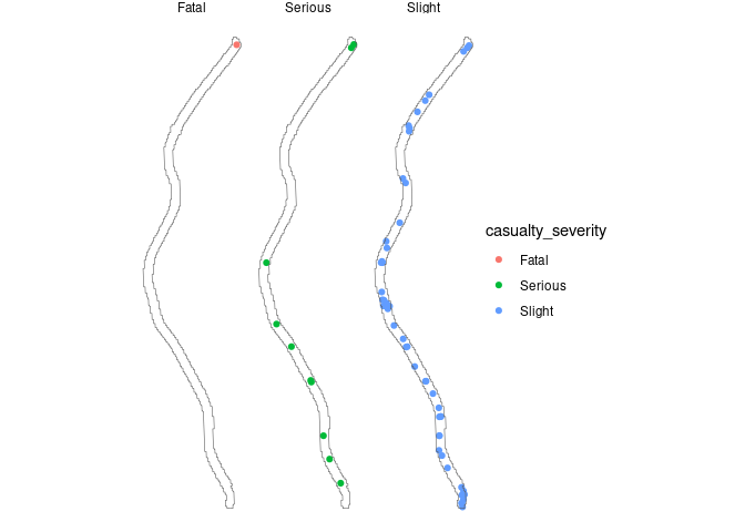
crashes_scott_hall = cas_sf[scott_hall_buffer, ]
ggplot(crashes_scott_hall) +
  geom_sf(aes(colour = casualty_severity)) +
  geom_sf(data = scott_hall_buffer, fill = NA) +
  facet_wrap(~casualty_severity) +
  theme_void()
We can output the data as follows:
st_write(crashes_scott_hall, "crashes_scott_hall.geojson", delete_dsn = TRUE)Deleting source `crashes_scott_hall.geojson' using driver `GeoJSON'
Writing layer `crashes_scott_hall' to data source
`crashes_scott_hall.geojson' using driver `GeoJSON'
Writing 64 features with 58 fields and geometry type Point.

