Convenient access to FVCOM datasets from R.
FVCOM produces ocean circulation models on an irregular mesh. Here is the user manual.
As an example, NECOFS leverages this mesh to deliver models for the Gulf of Maine, Mass coastal waters and a small number of estuaries. NECOFS provides an interactive web map
There are a number of models with a Gulf of Maine bend including both forecasts and data assimilative hindcasts.
Gulf of Maine forecasts are are available up to three days out. These are also archived and can be accessed for the time period of 2016-2023. NECOFS Forecast Archives
Regional hindcasts are another data product available on the SMAST NECOFS THREDDS Catalog. These may be used as proxies for real-world data which may otherwise not be available across these spatial scales or at hourly/daily timesteps.
Hindcast data is available beginning in 1978, but its coverage currently ends at different points in time dependent on the output timestep:
Version Note: Depending on which timestep is desired, the FVCOM mesh used after 2016 will vary between some combination of GOM4 and GOM5 mesh versions. These newer versions increase the number of mesh nodes and in the case of GOM5 increase the spatial extent of the model.
devtools::install_github("BigelowLab/fvcom")
Data are served via OPeNDAP on a THREDDS server THREDDS servers blend a simple user-navigable interface (similar to a file browser) with a machine readable data XML map Note the change in the file extension. Files served this way permit the user to treat the product as if it were a local file, allowing selective downlaod and access in a familar NetCDF format with needing to download the entire file.
NECOFS has it’s own THREDDS directory including a subdirectory for the GoM FVCOM models.
library(sf)
library(fvcom)
library(ncdf4)
library(dplyr)
Open the FVCOM resource as you would any NetCDF file.
library(fvcom)
library(ncdf4)
uri_base <- "http://www.smast.umassd.edu:8080/thredds/dodsC/models/fvcom/NECOFS/Archive/NECOFS_GOM/2019"
uri <- file.path(uri_base, "gom4_201901.nc")
x <- nc_open(uri)
# x
#      ...
#      53 variables (excluding dimension variables):
#         ...blah...
#         float lon[node]
#             long_name: nodal longitude
#             standard_name: longitude
#             units: degrees_east
#         float lat[node]
#             long_name: nodal latitude
#             standard_name: latitude
#             units: degrees_north
#         float xc[nele]
#             long_name: zonal x-coordinate
#             units: meters
#         float yc[nele]
#             long_name: zonal y-coordinate
#             units: meters
#         ...
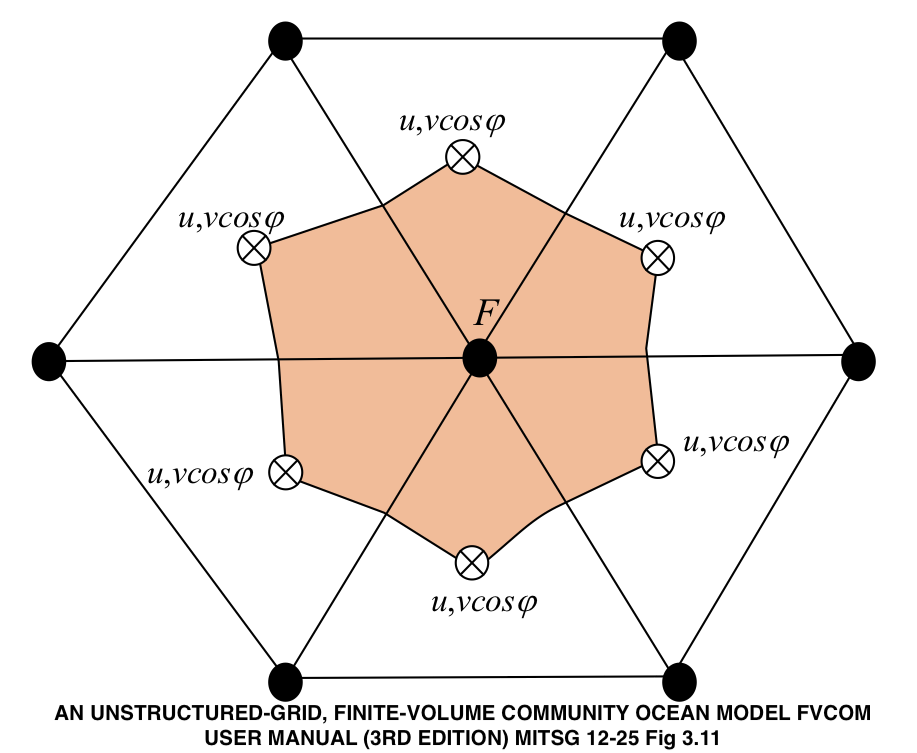
The mesh is defined by non-intersecting triangular elements bounded by
three nodes. Nodes are shown below as the solid dots, three nodes define
the boundary of element. Scalar values, like temperature, salinty and
height are defined at nodes. Vector values, such as velocity are defined
at the element centroids. Within the NetCDF object you can make complete
identification by examining which variables use the node dimensions
versus those that use the nele dimension.
Use the functions fvcom_nodes and fvcom_elems to extract location
information as either xy or lonlat pairs. Note we get both xy and
lonlat here for nodes. The same can be had for elements.
dplyr::left_join(fvcom::fvcom_nodes(x, what = 'lonlat'),
                 fvcom::fvcom_nodes(x, what = 'xy'), by = "node")
# Joining, by = "node"

# # A tibble: 53,087 x 5
#     node   lon   lat       x       y
#    <int> <dbl> <dbl>   <dbl>   <dbl>
#  1     1 -59.8  46.1 1699880 420500
#  2     2 -59.8  46.1 1705180 414890
#  3     3 -59.7  46.0 1709910 409690
#  4     4 -59.6  46.0 1715778 403368.
#  5     5 -59.6  45.9 1722603 395907
#  6     6 -59.5  45.8 1730039 387611.
#  7     7 -59.4  45.7 1737004 380188.
#  8     8 -59.3  45.7 1744943 371707.
#  9     9 -59.2  45.6 1752036 363693
# 10    10 -59.1  45.5 1761284 353679.
# # … with 53,077 more rows
Retrieving the timestamps provides you with a choice for assumptions you want to make about the hourly model output. Timestamps stored internally do not land on each hour.
head(fvcom_time(x, internal = TRUE), n = 6)
# [1] "1978-01-01 00:00:00 UTC" "1978-01-01 01:01:52 UTC"
# [3] "1978-01-01 01:58:07 UTC" "1978-01-01 03:00:00 UTC"
# [5] "1978-01-01 04:01:52 UTC" "1978-01-01 04:58:07 UTC"
We can get a proxy for these times, but prettily settled on each hour. The choice is yours.
head(fvcom_time(x, internal = FALSE), n = 6)
# [1] "1978-01-01 00:00:00 UTC" "1978-01-01 01:00:00 UTC"
# [3] "1978-01-01 02:00:00 UTC" "1978-01-01 03:00:00 UTC"
# [5] "1978-01-01 04:00:00 UTC" "1978-01-01 05:00:00 UTC"
Variables (the oceanographic ones) can be extract by node or element. It is possible to select a subset, but the operation on the whole dataset is quick and it is just as easy to subset after you have the table in hand.
v <- get_node_var(x, var = 'zeta')
# # A tibble: 48,451 × 2
#     node    zeta
#    <int>   <dbl>
#  1     1 -0.0131
#  2     2 -0.0392
#  3     3  0.0201
#  4     4  0.0450
#  5     5  0.0464
#  6     6  0.0158
#  7     7 -0.0143
#  8     8 -0.0270
#  9     9 -0.0377
# 10    10 -0.0539
# # … with 48,441 more rows
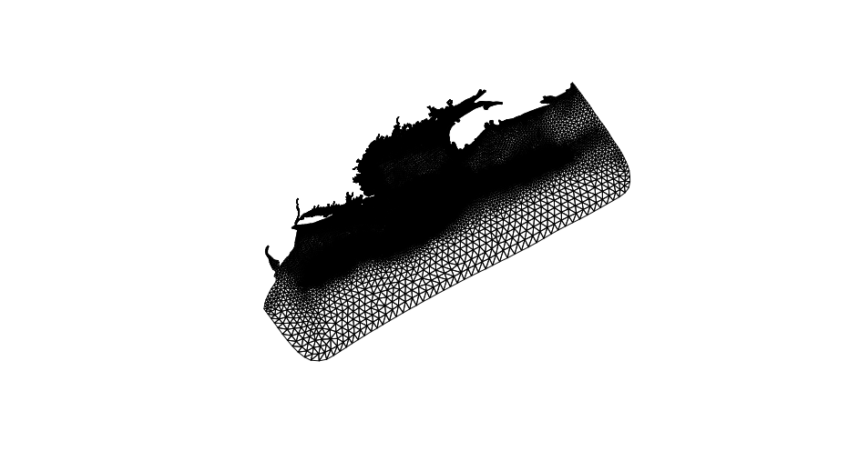
Some computation is required (not a lot) to produce the mesh which is comprised of non-intersecting polygons (triangles). Meshes can be derived from the lists of nodes or the list of elements. We have chosen to use elements by default as they are simple to construct from the adjancency lists provided in the NetCDF resource.
The each element in the mesh is defined by the three nodes identified by index, “p1”, “p2” and “p3”. The geometry is defined by either “lonlat” coordinates or projected mercator coordinates, “xy”.
mesh <- get_mesh_geometry(x, what = 'lonlat')
mesh
# Simple feature collection with 90415 features and 3 fields
# Geometry type: POLYGON
# Dimension:     XY
# Bounding box:  xmin: -75.68433 ymin: 35.28387 xmax: -56.8508 ymax: 46.14595
# Geodetic CRS:  WGS 84
# # A tibble: 90,415 × 4
#       p1    p2    p3                                                                 # geometry
#  * <int> <int> <int>                                                            <POLYGON # [°]>
#  1     1   196   197 ((-59.8902 46.09442, -59.82598 46.0583, -59.8746 46.0069, -59.8902 # 46.0…
#  2     1     2   196 ((-59.8902 46.09442, -59.81069 46.14595, -59.82598 46.0583, -59.8902 # 46…
#  3   196     2     3 ((-59.82598 46.0583, -59.81069 46.14595, -59.75268 46.09011, # -59.82598 …
#  4     4   196     3 ((-59.70132 46.03855, -59.82598 46.0583, -59.75268 46.09011, # -59.70132 …
#  5   196     4   195 ((-59.82598 46.0583, -59.70132 46.03855, -59.78878 46.00403, # -59.82598 …
#  6   195     4   194 ((-59.78878 46.00403, -59.70132 46.03855, -59.72971 45.94034, # -59.78878…
#  7     5   194     4 ((-59.63753 45.9757, -59.72971 45.94034, -59.70132 46.03855, # -59.63753 …
#  8     5   193   194 ((-59.63753 45.9757, -59.65802 45.86837, -59.72971 45.94034, # -59.63753 …
#  9   193     5     6 ((-59.65802 45.86837, -59.63753 45.9757, -59.56369 45.90162, # -59.65802 …
# 10   192   193     6 ((-59.59155 45.78925, -59.65802 45.86837, -59.56369 45.90162, # -59.59155…
# # … with 90,405 more rows
plot(sf::st_geometry(mesh))
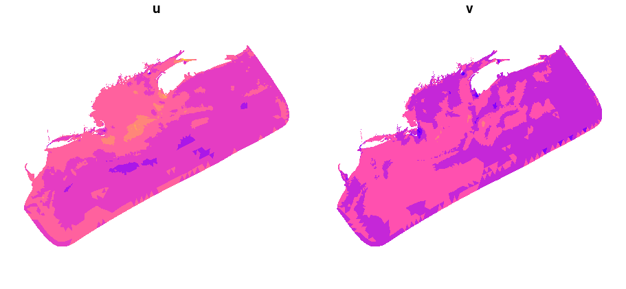
We can assign variable values to the polygons by reusing the mesh table. These variables are associated with either node or elements. If node-referenced variables are requested the mean of three neighboring nodes (which define an element) is computed. Where element-referenced variables are requested no averaging is done - the values are simply assigned to the mesh element.
mesh <- get_mesh(x, vars = c("zeta", "u", "v"), mesh = mesh)
# Simple feature collection with 90415 features and 6 fields
# Geometry type: POLYGON
# Dimension:     XY
# Bounding box:  xmin: -75.68433 ymin: 35.28387 xmax: -56.8508 ymax: 46.14595
# Geodetic CRS:  WGS 84
# # A tibble: 99,137 x 7
#          v        u    zeta    p1    p2    p3                 geometry
#      <dbl>    <dbl>   <dbl> <int> <int> <int>            <POLYGON [°]>
#  1 -0.0333 -0.0275  -0.0224    96     1    95 ((-59.8902 46.09441, ...
#  2 -0.0867  0.0217  -0.0188    95     1     2 ((-59.82597 46.0583, ...
#  3 -0.0588  0.00963 -0.0280     3    95     2 ((-59.70132 46.03855,...
#  4 -0.122  -0.0108  -0.0404    95     3    97 ((-59.82597 46.0583, ...
#  5 -0.0883 -0.0362  -0.0494    97     3    98 ((-59.78879 46.00403,...
#  6 -0.110  -0.0200  -0.0460     4    98     3 ((-59.63753 45.97571,...
#  7 -0.0751 -0.0659  -0.0639     4    99    98 ((-59.63753 45.97571,...
#  8 -0.0750 -0.00269 -0.0631    99     4     5 ((-59.65802 45.86837,...
#  9 -0.0518 -0.0552  -0.0796   100    99     5 ((-59.59155 45.78925,...
# 10 -0.0501  0.00748 -0.0800     5     6   100 ((-59.56369 45.90162,...
# # … with 99,127 more rows
plot(mesh[c("u", "v")], lty = 'blank', main = c("u", "v"))
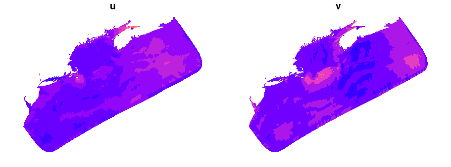
You can request variables at various dimensions such as times and sigma
levels/layers - the default is the first of each dimension. While you
can request one of these in ‘real’ values (such as POSIXct time), you
can also provide a 1-based index into that dimension. The example below
requests the same variables as above but at the 24th time interval. See
the functions get_node_var and get_elem_var for details.
mesh <- get_mesh(x, vars = c("zeta", "u", "v"), mesh = mesh, time = 24)
# Simple feature collection with 90415 features and 6 fields
# Geometry type: POLYGON
# Dimension:     XY
# Bounding box:  xmin: -75.68433 ymin: 35.28387 xmax: -56.8508 ymax: 46.14595
# Geodetic CRS:  WGS 84
# # A tibble: 99,137 x 7
#         v      u  zeta    p1    p2    p3                                             geometry
#     <dbl>  <dbl> <dbl> <int> <int> <int>                                        <POLYGON [°]>
#  1 0.148  0.122  0.451    96     1    95 ((-59.8902 46.09441, -59.81069 46.14595, -59.82597 …
#  2 0.313  0.0446 0.435    95     1     2 ((-59.82597 46.0583, -59.81069 46.14595, -59.75268 …
#  3 0.191  0.0131 0.409     3    95     2 ((-59.70132 46.03855, -59.82597 46.0583, -59.75268 …
#  4 0.105  0.0295 0.400    95     3    97 ((-59.82597 46.0583, -59.70132 46.03855, -59.78879 …
#  5 0.150  0.116  0.382    97     3    98 ((-59.78879 46.00403, -59.70132 46.03855, -59.72971…
#  6 0.101  0.0564 0.375     4    98     3 ((-59.63753 45.97571, -59.72971 45.94034, -59.70132…
#  7 0.143  0.144  0.377     4    99    98 ((-59.63753 45.97571, -59.65802 45.86837, -59.72971…
#  8 0.0536 0.0679 0.371    99     4     5 ((-59.65802 45.86837, -59.63753 45.97571, -59.56369…
#  9 0.157  0.119  0.373   100    99     5 ((-59.59155 45.78925, -59.65802 45.86837, -59.56369…
# 10 0.0470 0.0627 0.366     5     6   100 ((-59.56369 45.90162, -59.48375 45.8194, -59.59155 …
# # … with 99,127 more rows
plot(mesh[c("u", "v")], lty = 'blank', main = c("u", "v"))
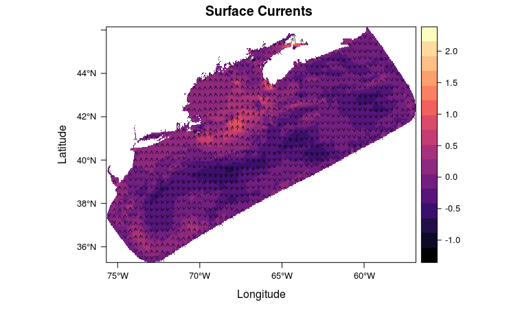
The mesh can be interpolated on to a regular grid (“rasterize”).
    uv <- raster::stack(sapply(c("u", "v"),
        function(f) {
            fvcom::rasterize(mesh, field = f)
        }, simplify = FALSE))
    rasterVis::vectorplot(uv, isField = 'dXY',
                          col.arrows = "white",
                         main = 'Surface Currents')
See this for a walk through.
