2D ( time independent) scalar field ( potential). Create vector field and draw field lines and equipotential lines
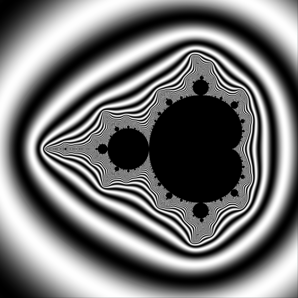
Exterior is coloured with potential ( grayscale)
p = log(potential)/K;
color = 255* (1+cos(TwoPi*p))/2.0;
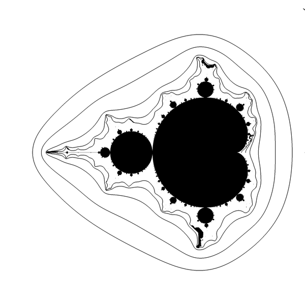
Exterior is white with black equipotential curves
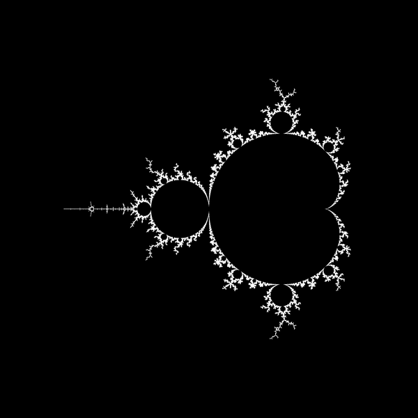
Boundary using noise detection
double BoundaryMeasure = 1.15; // higher value = thinner boundary
// FindBoundary
if (NoiseMeasure> BoundaryMeasure) A[i] = 255 ;	// white
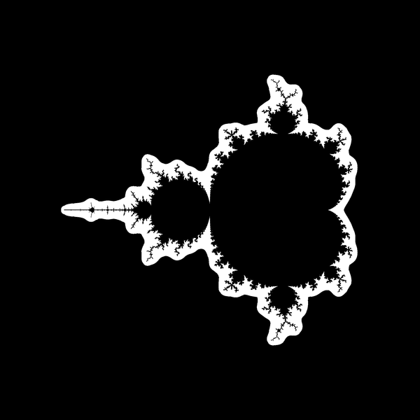
Noise pixels
double NoiseMeasureThreshold = 0.045; // arbitrary for c = 0.365000000000000  +0.000000000000000 i    period = 0
//  FindNoisyPixels
if (NoiseMeasure> NoiseMeasureThreshold) A[i] = 255 ; // whitehere field lines are external rays
- do not cross with each other but 2 or more lines may land on the same point ( root or Misiurewicz point)
- are perpendicular ( normal) to equipotential lines = are gradient lines of potential ( scalar field)
memory is OK

real	0m28,965s
user	3m47,483s
sys	0m0,092s

render image = compute and write image data bytes to the array
File 10_89990.pgm saved.
ClearExterior =  make exterior solid color = white
 exterior p = 0.751188

draw equipotential curve thru point c = (0.9000000000000000; 0.0000000000000000) pixel = (1916, 1000)
 	start point
	for c = (0.900000;0.000000)	noise measure = 0.0025952006903814	potential = 0.9901006463279854
	c is inside the array : iy = 1916 iy = 1000	and outside M set
	end point	ix = 1916 iy = 1000 i = 2001916 potential = 0.9901033608952807
	curve is closed = stop ( good) after 4357 steps (pixels)


draw equipotential curve thru point c = (0.7000000000000000; 0.0000000000000000) pixel = (1805, 1000)
 	start point
	for c = (0.700000;0.000000)	noise measure = 0.0045160797467720	potential = 0.5989907665960282
	c is inside the array : iy = 1805 iy = 1000	and outside M set
	end point	ix = 1805 iy = 1000 i = 2001805 potential = 0.5989911428328348
	curve is closed = stop ( good) after 3825 steps (pixels)


draw equipotential curve thru point c = (0.5000000000000000; 0.0000000000000000) pixel = (1694, 1000)
 	start point
	for c = (0.500000;0.000000)	noise measure = 0.0111195774508909	potential = 0.2128012374973248
	c is inside the array : iy = 1694 iy = 1000	and outside M set
	end point	ix = 1694 iy = 1000 i = 2001694 potential = 0.2127903458916913
	curve is closed = stop ( good) after 3687 steps (pixels)


draw equipotential curve thru point c = (0.4000000000000000; 0.0000000000000000) pixel = (1638, 1000)
 	start point
	for c = (0.400000;0.000000)	noise measure = 0.0244119823222931	potential = 0.0632189280903892
	c is inside the array : iy = 1638 iy = 1000	and outside M set
	end point	ix = 1638 iy = 1000 i = 2001638 potential = 0.0631906592052049
	curve is closed = stop ( good) after 4125 steps (pixels)

File 10_89980.pgm saved.
Find boundary of Mandelbrot set using  noise measure
File 10_89970.pgm saved.
Find noisy pixels
File 10_89960.pgm saved.
for c = (0.000000;0.000000)	noise measure = 0.0000000000000000	potential = 0.0000000000000000
for c = (0.100000;0.000000)	noise measure = 0.0000000000000000	potential = 0.0000000000000000
for c = (0.200000;0.000000)	noise measure = 0.0000000000000000	potential = 0.0000000000000000
for c = (0.250000;0.000000)	noise measure = 0.2500000000000000	potential = 0.0000000000000000
for c = (0.260000;0.000000)	noise measure = 3.1457717601949291	potential = 0.0000000019934531
for c = (0.270000;0.000000)	noise measure = 0.5572597205697883	potential = 0.0000044162911707
for c = (0.280000;0.000000)	noise measure = 0.3078640888246843	potential = 0.0000587486278177
for c = (0.290000;0.000000)	noise measure = 0.1872334952074938	potential = 0.0003708182242248
for c = (0.300000;0.000000)	noise measure = 0.1290122547411083	potential = 0.0012438403001236
for c = (0.350000;0.000000)	noise measure = 0.0457918910257952	potential = 0.0183838747379665
for c = (0.400000;0.000000)	noise measure = 0.0244119823222931	potential = 0.0632189280903892
for c = (0.450000;0.000000)	noise measure = 0.0156374406145566	potential = 0.1305368896713344
for c = (0.500000;0.000000)	noise measure = 0.0111195774508909	potential = 0.2128012374973248
for c = (0.600000;0.000000)	noise measure = 0.0066430404569894	potential = 0.3984187631443595
for c = (0.700000;0.000000)	noise measure = 0.0045160797467720	potential = 0.5989907665960282
for c = (0.800000;0.000000)	noise measure = 0.0033359942064616	potential = 0.7958924429230689
for c = (0.900000;0.000000)	noise measure = 0.0025952006903814	potential = 0.9901006463279854
for c = (1.000000;0.000000)	noise measure = 0.0020908718498594	potential = 1.1743374869011141


Parameter plane with Mandelbrot set
corners: CxMin = -2.550000	CxMax = 1.050000	 CyMin = -1.800000	 CyMax 1.800000
corners: ixMin = 0	ixMax = 1999	 iyMin = 0	 iyMax 1999
exterior = CPM/M
IterationMax = 90000
EscapeRadius = 10
iPixelRadius = ixMax* 0.002 = 1 so big pixel = 4 (small) pixels
Why real time is lower then user time ?
- dimension : 2D / 3D / ...
- input
- trace a curve in the array of precomputed values ( read value of new point from the array). Array = image
- trace a curve in complex 2D plane ( compute each point)
- curve types
- closed / not closed ( ray)
- simple,
- critical points / singularities
- grid
- structured / unstructured
- quadratic / triangular ( Coxeter-Freudenthal decomposition (triangulation))
- pixel connectivity
- stoping criteria
- boundary of the Grid ( image)
- maximal curve length
- Maximum compute time
- trace
- forward / backward or clockwise/counterclockwise
- how many seed points
- fixed step / change
- algorithm
Input:
- plane (parameter plane or dynamic plane)
- scalar function ( potential)
- vector function
Steps:
- create scalar field using scalar function ( potential)
- create vector field from scalar field using vector function ( gradient of the potential)
- compute/draw :
- filed lines ( stream lines )
- contour lines ( [[Fractals/Iterations_in_the_complex_plane/equipotetential|equipotential lines]] )
- map whole field using Line Integral Convolution (LIC)
tracing a curve means compute successive points on the curve, one by one, until stopping criteria are met
graph TD
A[Start point] --> B(Compute next point)
B --> C{meet stop criteria ? }
C --> |No|B
C -->|Yes| D[End]
Tracing a curve on the triangular grid
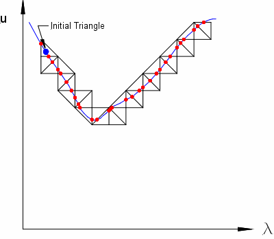
Image by Michael E. Henderson
"scanning means to check every pixel". Other names : detection, extraction
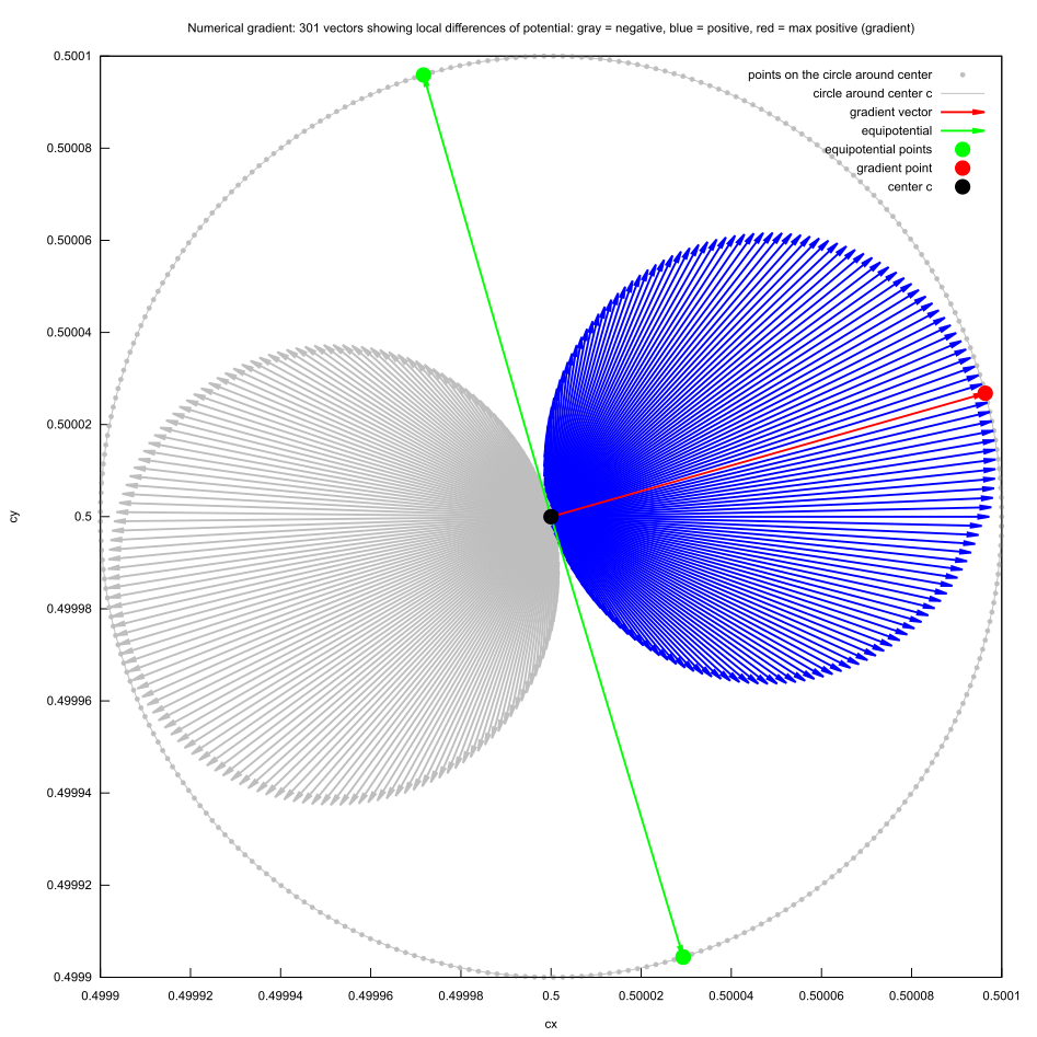
Gradient
- The gradient of a scalar field is a vector that represents the magnitude and the direction of the greatest increase rate of the field
- s.c - trace equipotential curves on the parameter plane ( my own code))
- boundary.c - Boundary Tracing Generation Method, traces the outline of areas of a single color and fills them in. Copyright (c) 1994-1997 Michael R. Ganss. All Rights Reserved.
- lines.c - detect-lines, extract lines and their width from images. Copyright (C) 1996-1998 Carsten Steger. from GRASP
- y.c - Mandelbrot boundary tracing example for Youtube video : Writing a Mandelbrot Fractal Renderer with Boundary Tracing Algorithm – © Joel Yliluoma
- jung.c - code by Wolf Jung (C) 2007-2017
- fractint.c - code for the bound_trace from fractint
- gradient.mac - Maxima CAS code for numerical aproximation of gradient, equiopotential direction and making images text output of the program
- grad_f.mac - Maxima CAS code for numerical aproximation of gradient
- mandelbrot-ex_ray-out
- dynamic_external_angle
- m_d_exray_in
- ray-backward-iteration
- NonInteractiveParameterRayInMPFR
- dynamic_ray_newton
- parameter_ray_in_newton_mpfr
- Argument tracing by Wolf Jung
- A Rasterizing Algorithm for Drawing Curves by Alois Zingl
- Meandering triangles ( marching triangles)
- Otis by Tomoki Kawahira
- Numerical_continuation
- Isoline
- CURVE TRACING AND CURVE DETECTION IN IMAGES by Karthik Raghupathy
- curve tracing algorithm, proposed by Steger
- Carsten Steger, “An unbiased detector of curvilinear structures,” IEEE Transactions on Pattern Analysis and Machine Intelligence, February 1998.
- Unbiased Extraction of Curvilinear Structures from 2D and 3D Images by Carsten Steger
- Curviliniar_Detector in matlab by Emmanouil Kapernaros
- Curve tracing by Eugene Katrukha and code
- Ridge (Line) Detection Plugin (Fiji) by Thorsten Wagner, Mark Hiner and code
- The process of subdividing an object (either geometric object, or a data structure) recursively until some criteria is met.
- Boundary Scanning by Robert P. Munafo
- How to “inform” successive ContourPlot calculations in Mathematica?
- wikipedia : Boundary_tracing
- The Boundary Tracing algorithm by Evgeny Demidov
- Fast Contour-Tracing Algorithm Based on a Pixel-Following Method for Image Sensors by Jonghoon Seo, et al.
- Tracing Boundaries in 2D Images by V. Kovalevsky
- the Moore-Neighbor tracing algorithm by Abeer George Ghuneim
- Square Tracing Algorithm by Abeer George Ghuneim
- conturs in OpenCV and Python
- Bisqwit
- Drawing M-set by contour lines method
- M. Romera, G. Pastor and F. Montoya, "Graphic Tools to Analyse One-Dimensional Quadratic Maps", Computers & Graphics, 20/2 (1996), 333-339
- M. Romera, G. Pastor and F. Montoya, "Drawing the Mandelbrot set by the method of escape lines", Fractalia, 5, n.º 17 (1996), 11-13.
- an explicit conformal isomorphism between the complement of the Mandelbrot set M and the complement of the closed unit disk D
- CONREC = A Contouring algorithm of some surface represented as a regular triangular mesh by Paul Bourke
code
- streamlines - The library by Andrei Kashcha, which builds streamlines for arbitrary vector fields, trying to keep uniform distance between them.
- fieldplay- by Andrei Kashcha
- How I built a wind map with WebGL by Vladimir Agafonkin
- HARSH BHATIA
- stackoverflow question: how-to-plot-streamlines-when-i-know-u-and-v-components-of-velocitynumpy-2d-ar
- stackoverflow question: how-to-create-streamline-like-arrow-lines-in-gnuplot
- wikipedia : Image-based_flow_visualization
- Robust Polylines Tracing for N-Symmetry Direction Field on Triangulated Surfaces by NICOLAS RAY and DMITRY SOKOLOV
- presentation by Abdelkrim Mebarki
- CGAL package by Abdelkrim Mebarki
- matplotlib
- math.stackexchange question: solving-for-streamlines-from-numerical-velocity-field/1950329#1950329
- Grid-Independent Detection of Closed Stream Lines in 2D Vector Fields by H. Theisel, T. Weinkauf, H.-C. Hege, H.-P. Seidel
- the Morse-Smale complex in python by Nithin Shivashankar.
- stackoverflow question: computing-and-drawing-vector-fields
- An external ray is an integral curve of the gradient vector field ∇G on Bc(∞).
- AN ACCURATE ALGORITHM FOR RASTERIZING ALGEBRAIC CURVES by Gabriel Taubin
- Visualizing Arcs of Implicit Algebraic Curves, Exactly and Fast by Pavel Emeliyanenko, Eric Berberich, Michael Sagraloff1
gradient = "direction and rate of fastest increase". If at a point p, the gradient of a function of several variables is not the zero vector
- the direction of the gradient is the direction of fastest increase of the function at p
- its magnitude is the rate of increase in that direction
discrete differential geometry
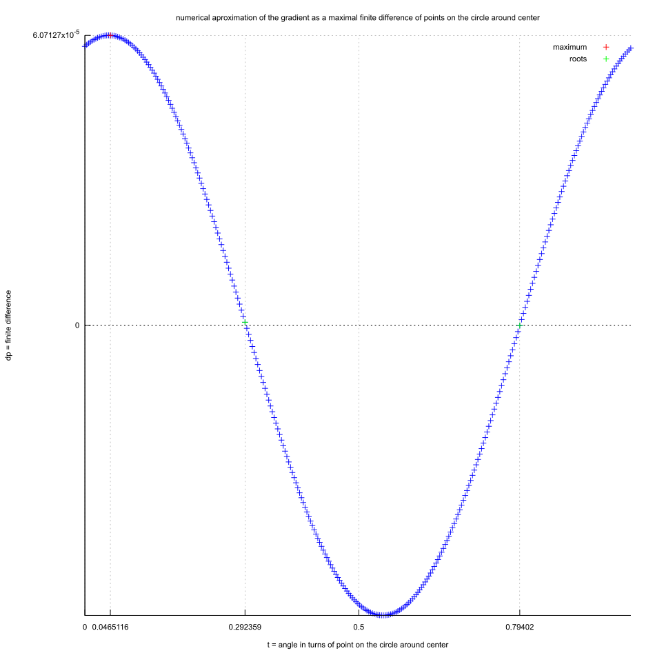
In 1D case derivative of the function f at point x gives the slope of the tangent line at the point x
It is aproximated by the maximal finite differnce:
In 2D case gradient (generalization of the derivative) of function f at point (x,y) gives the slope of the plane (flat surface) tangent to the 3D surface z = f(x,y)
- Numerical Differentiation in two variables ( complex number = x+y*i) by approximation by centered finite differences scheme
Finite-Difference Method = FDM
Example code : "gradient direction computation based on image brightness. I've made a matrix bright[width][height] containing brightness values for every pixel of the image"
	// https://stackoverflow.com/questions/4003615/gradient-direction-computation
   double grad_x(int x,int y){
    	if(x==width-1 || x==0) return bright[x][y];
    	return bright[x+1][y]-bright[x-1][y];
    }
    double grad_y(int x,int y){
    	if(y==height-1 || y==0) return bright[x][y];
    	return bright[x][y+1]-bright[x][y-1];
}Different outputs of numerical gradient function:
- angle of the gradient vector (and the radius )
- point directed by the gradient vector
Modifications:
- Adaptive step size
- Corner cases Description by Nils Pipenbrinck
The corner cases are a problem because you don't have enough data to calculate a gradient in the same way as the other pixels. One way to deal with them is to simply not calculate the corner cases and live with a slightly smaller image.
If this is not an option you can also extrapolate the missing data. If you assume that the gradient changes smoothly it works like this:
In your x-gradient calculations you may have calculated the derivate A for pixel 1 and B for pixel 2. If you want to extrapolate a value for pixel 0 (the corner case) the value a-(b-a) could be used.
pixel1: gradient = 100 pixel2: gradient = 80
extrapolate using a-(b-a):
pixel0: gradient = 100 - (80-100)) = 120
Links:
- math.stackexchange question: how-to-approximate-numerically-the-gradient-of-the-function-on-a-triangular-mesh
- Numerical differentiation by Gonzalo Galiano Casas and Esperanza Garcia Gonzalo
- gradient of the potential by Linas Vepstas
- PYTHON LABS by Gonzalo Galiano Casas and Esperanza García Gonzalo
- Finite-difference approximation by Tim Vieira
- wikipedia : Finite_difference
Methods
- Euler ( a first order method = RK1)
- Midpoint ( a second order method)
- Runge-Kutta methods = RK4
- Adaptive Distance Grid Based Algorithm for Farthest Point Seeding Streamline Placement by Abdelkrim Mebarki -"use the Runge-Kutta second order integration scheme to construct the polyline for approximating our streamline."
- the Runge-Kutta of 4th order method = RK4
- 1D - numerical integration by Glenn Fiedler
- 2D - Runge–Kutta 4 integrator by Marek Fišer
- An Intuitive Description of Runge-Kutta Integration by Daren Scot Wilso
- stackoverflow question : runge-kutta-rk4-integration-for-game-physics
- parameter_external_angle/tavis.cpp tavis.cpp
- The Runge-Kutta Method for 2-Dimensional Systems
- discrete differential geometry ** mesh
- Digital Topology
- digital image processing
- binary 2D image
- discrete complex dynamics
- complex quadratic polynomial
- parameter plane
- lines tangent and normal to curve at a point
- trace
- a curve
- a boundary
- a contour
- polylines
- curve
- isocurve ( isoline): equipotential curve
- Fields
- 2D scalar field
- gradient
- Visualizing the Variability of Gradients in Uncertain 2D Scalar Fields by Tobias Pfaffelmoser, Mihaela Mihai and Rudiger Westermann
- Array computing and curve plotting (in python) by Hans Petter Langtangen
- Visualization of scalar and vector fields ( in matlab) by Øyvind Ryan, Hans Petter Langtangen
- visualization-with-matlab
- Simulating Gradient Contour and Mesh of a Scalar Field ( in Matlab) by Usman Ali Khan, Bismah Tariq, Khalida Raza, Saima Malik, Aoun Muhammad
- chebfun is an open-source software system for numerical computing with functions.
- Paraview
- A streamline is an integral curve of the vector field
- quiver plot: plot of the 2-D vector field ( vectors as arrows with components (u,v) at the points (x,y) )
- gradient
- numerical differentiation = numerically computing the gradient of a function
- Mathematical optimization = finding numerically minimums (or maximums or zeros) of a function
- FLOW VISUALIZATION
- 2D Velocity Fields
- Applications:
- streamline tracing on triangular and quadrilateral grids
- Numerical continuation
- Simplicial or piecewise linear continuation
- Visualization of Algebraic Curves - curve sketching
GitLab uses:
- the Redcarpet Ruby library for Markdown processing
- KaTeX to render math written with the LaTeX syntax, but only subset. Here is used version
cd existing_folder
git init
git remote add origin git@gitlab.com:adammajewski/curve-tracing.git
git add .
git commit -m "Initial commit"
git push -u origin master
mkdir images
git add *.png
git mv  *.png ./images
git commit -m "move"
git push -u origin master
then link the images:

gitm mv -f
Local repo : ~/c/mandel/p_e_angle/trace_last/test5
