adamrb/p3-benchmarking

Accelerating Deep Learning Training with P3's and V100

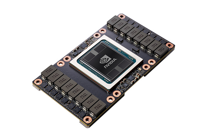
This lab will walk you through a few benchmark tests to understand TensorFlow and MXNet performance on the p3 platform.

Launch the AMI

1. From the instance launch screen, choose the "Deep Learning AMI (Amazon Linux) Version 7.0". In us-west-2, this is ami-e42f499c.
2. Choose a "p3.2xlarge" instance
3. Launch in any Subnet & Security Group with public SSH access

Comparing throughput of FP16 to FP32 calculations

For the first test, we're going to compare the performance of TensorFlow when using 32-bit and 16-bit variable lengths. 32 bit (single precision or FP32) and even 64-bit (double precision or FP64) floating point variables are popular for many applications that require high prececision. These are workloads like engineering simulations where you're simulating real world behavior and need the mathemtical models to be as exact as possible. However, deep learning is more resiliant to lower precision due to the way that backpropagaion algorithms work. Many people find that the reduction in memory usage and increase in speed gained by moving to half or mixed precision (16-bit or FP16) are worth the minor trade offs in accuracy.

Let's test the performance difference we get when running in FP32 vs FP16.

1. Log into the instance and CD to the home directory

cd ~/

2. Activate the TensorFlow conda environment

source activate tensorflow_p36

3. Clone the GitHub repo for Tensorflow examples and benchmarking code

git clone --recursive https://github.com/tensorflow/benchmarks.git tf-benchmark-src

4. Change to the benchmarking directory

cd tf-benchmark-src/scripts/tf_cnn_benchmarks/

5. Run the 32-bit benchmark

python tf_cnn_benchmarks.py --variable_update=replicated --model=resnet50 --batch_size=128 --num_batches=100 --loss_type_to_report=total_loss --num_gpus=1 --single_l2_loss_op=True --local_parameter_device=cpu --all_reduce_spec=pscpu

We're looking for the throughput number in order to measure performance. You should see a number around 400 samples/second.

If you'd like to view the CPU usage while this is running, you can run "nvidia-smi" from another terminal while it's running.

6. Run the 16-bit (mixed precision) benchmark

Now let's see what happens when we change the precision from the default 32-bit, to the 16-bit supported on the V100 GPU. Note that we can increase the batch size because FP16 requires less memory.

python tf_cnn_benchmarks.py --variable_update=replicated --model=resnet50 --batch_size=256 --use_fp16=True --num_batches=100 --loss_type_to_report=total_loss --num_gpus=1 --single_l2_loss_op=True --local_parameter_device=cpu --all_reduce_spec=pscpu

By taking advantage of the mixed precision capabilities introduced in Pascal (and also available in Volta), you can see we're doubling the throughput.

Running a full ImageNet training

Now we're going to actually train an image classification neural network with the ImageNet dataset (http://www.image-net.org/) using MXNet

1. Log into the instance and CD to the home directory

cd ~/

2. Activate the MXNet conda environment

source activate mxnet_p36

3. Export the CUDNN autotune environment variable to allow MXNet to discover the best convolution algorithm

export MXNET_CUDNN_AUTOTUNE_DEFAULT=2

4. Create a directory where you'll be working

mkdir -p ~/data && cd ~/data

5. Configure the AWS CLI to use more parallel threads

aws configure set default.s3.max_concurrent_requests 20

5. Copy the training and validation data locally

6. Download the training source code

cd ~/ && git clone --recursive https://github.com/apache/incubator-mxnet.git mxnet-src

7. Create an index file from the source data to enable random access

python ~/mxnet-src/tools/rec2idx.py ~/data/imagenet1k-val.rec ~/data/imagenet-val.idx

python ~/mxnet-src/tools/rec2idx.py ~/data/imagenet1k-train.rec ~/data/imagenet-train.idx

The second command should take about 25 seconds.

8. Run the full training

time python ~/mxnet-src/example/image-classification/train_imagenet.py \
  --gpu 0 --batch-size 224 \
  --data-train ~/data/imagenet1k-train.rec --data-val ~/data/imagenet1k-val.rec\
  --disp-batches 100 --network resnet-v1 --num-layers 50 --data-nthreads 40 \
  --min-random-scale 1.5 --max-random-shear-ratio 0.15 --max-random-rotate-angle 0 \
  --max-random-h 0 --max-random-l 0 --max-random-s 0 --dtype float16 \
  --num-epochs 1 --kv-store nccl

This is going to take a significant amount of time (about 30 minutes). We're training a convolutional neural network (resnet) with a dataset consisting of 1,000,000 labeled images depicting 1,000 object categories. You can see the accuracy of predictions increasing the more data that's being trained by the model. We're only allowing it to go through 1 epoch, which means we're just doing one pass of all of the data. For better accuracy, you will need to run multiple passes.

Running this same training on a p3.16xlarge takes about 5 minutes and trains at around 5,800 images a second. It takes roughly 30 minutes to train 10 epochs to a validation accuracy of 48%. You can look to further optimize this by changing the learning rate, batch size, number of layers, and network.