When you enter the monthly sales data of your products in the past two years, our application reports how much your product will be sold for each month of the next two years with 4 different forecasting methods. These forecasting methods are "Exponential Smoothing","Double Exponential Smoothing","Regression Analysis" and "Deseasonalized Regression Analysis". MSE is calculated for each method and the method with the lowest error rate is determined. But you can get the reports of all other forecasting methods.
Our application has a user-friendly interface. We used the JavaFX library in the interface of our application and benefited from FXML technology. Besides, we preferred to use MongoDB in our program because of its flexibility, speed, power and compatibility with Java. It is very enjoyable to make the database management part of our application from MongoDB Atlas. Atlas made it very easy to deal with the database, thanks to its cool and understandable interface.
The main screen of our application is shown above. When we add the datasets, the naming of the dataset is done according to the date added by the application. But we changed the names two datasets (Dataset 1 and Dataset 2) from the database later, making it easier to read.
When we select a dataset from the main screen and press the View/Update button, we are greeted with a screen where we can see the records in the dataset more clearly and perform operations on it.
If you enter a wrong record while adding a dataset, there is no need to delete the dataset and create a record again. In view/update menu datasets, each record is contained in an editable text field. In the example above, we updated the record from 300 to 300000.
Above, we see that this update is also made automatically from the database.
While we are in the database, let's talk about how the data is stored here. As seen in the figure above, each of our dataset is stored with a unique id named "_id". As we mentioned before, the naming of the dataset is done according to the added date. This name is stored in the "Name" key in the database. Since we know that each dataset will contain two years of data, we have stored these records in our model in arrays named "First Year" and "Second Year". Records of each month are kept in these arrays. Note that the records of these months are also kept in array type. We do this because we want to have the flexibility of having more than one record per month. Thus, when adding a dataset, the user can add not only 30 days of data, but also 10, 15 or even 1 day data. How many records each month consists of is also stored in the database in the key named "Number of Records for Each Month". In our JAVA program, we first need this value for our forecast process.
When you click the "Add" button on our main screen, you will be directed to a screen where you can easily add datasets.
If there is no problem with the dataset you want to add, the dataset will be added to both the main page table and the database.
If you click the "Delete" button, the selected dataset will be deleted instantly from both the dataset table and the database.
When you select a dataset on the main page and click the "Get forecast" button, you will be directed to a page with the forecast methods of the dataset you selected.
In the menu shown in figure above, s"Min Forecasted Sales", "Max Forecasted Sales" and "MSE" of the forecasted datasets created with “Exponential Smoothing”, “Double Exponential Smoothing”, “Regression Analysis” and “Deseasonalised Regression Analysis” methods are shown for the selected dataset. Below this table, the most appropriate method for the selected dataset according to the MSE comparison is indicated (The method with the lowest MSE value is recommended).
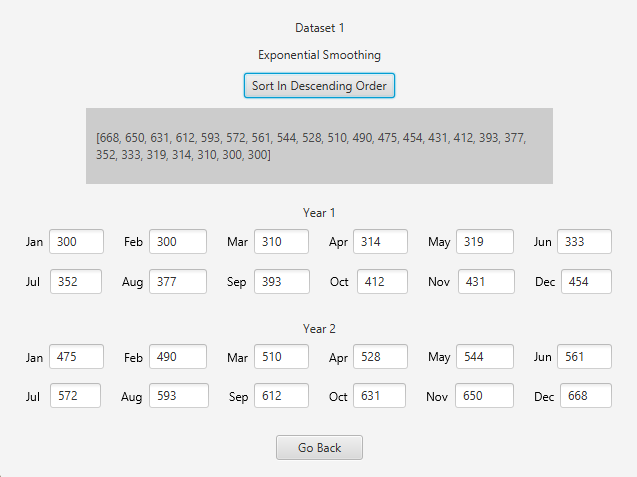
After selecting a method from this table, when you click on the "Get Forecasted Dataset" button, you can see the sales forecast values for the next two years using the method you selected.
Below are the sales forecasts for the next two years for all methods for "Dataset 1".


