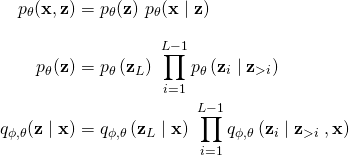
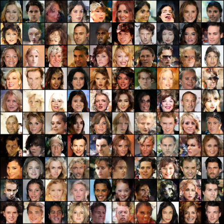
PyTorch implementation of Ladder Variational Autoencoders (LVAE) [1]:
where the variational distributions q at each layer are multivariate Normal with diagonal covariance.
Significant differences from [1] include:
- skip connections in the generative path: conditioning on all layers above rather than only on the layer above (see for example [2])
- spatial (convolutional) latent variables
- free bits [3] instead of beta annealing [4]
pip install -r requirements.txt
CUDA_VISIBLE_DEVICES=0 python main.py --zdims 32 32 32 --downsample 1 1 1 --nonlin elu --skip --blocks-per-layer 4 --gated --freebits 0.5 --learn-top-prior --data-dep-init --seed 42 --dataset static_mnist
Dependencies include boilr (a framework for PyTorch) and multiobject (which provides multi-object datasets with PyTorch dataloaders).
Log likelihood bounds on the test set (average over 4 random seeds).
| dataset | num layers | -ELBO | - log p(x) ≤ [100 iws] |
- log p(x) ≤ [1000 iws] |
|---|---|---|---|---|
| binarized MNIST | 3 | 82.14 | 79.47 | 79.24 |
| binarized MNIST | 6 | 80.74 | 78.65 | 78.52 |
| binarized MNIST | 12 | 80.50 | 78.50 | 78.30 |
| multi-dSprites (0-2) | 12 | 26.9 | 23.2 | |
| SVHN | 15 | 4012 (1.88) | 3973 (1.87) | |
| CIFAR10 | 3 | 7651 (3.59) | 7591 (3.56) | |
| CIFAR10 | 6 | 7321 (3.44) | 7268 (3.41) | |
| CIFAR10 | 15 | 7128 (3.35) | 7068 (3.32) | |
| CelebA | 20 | 20026 (2.35) | 19913 (2.34) |
Note:
- Bits per dimension in brackets.
- 'iws' stands for importance weighted samples. More samples means tighter log likelihood lower bound. The bound converges to the actual log likelihood as the number of samples goes to infinity [5]. Note that the model is always trained with the ELBO (1 sample).
- Each pixel in the images is modeled independently. The likelihood is Bernoulli for binary images, and discretized mixture of logistics with 10 components [6] otherwise.
- One day I'll get around to evaluating the IW bound on all datasets with 10000 samples.
- Statically binarized MNIST [7], see Hugo Larochelle's website
http://www.cs.toronto.edu/~larocheh/public/datasets/ - SVHN
- CIFAR10
- CelebA rescaled and cropped to 64x64 – see code for details. The path in
experiment.data.DatasetLoaderhas to be modified - binary multi-dSprites: 64x64 RGB shapes (0 to 2) in each image
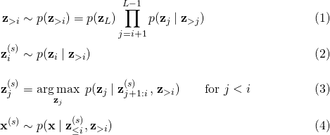
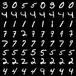
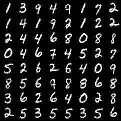
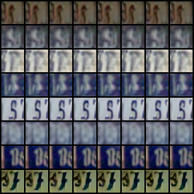
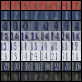
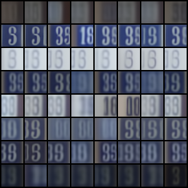
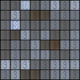
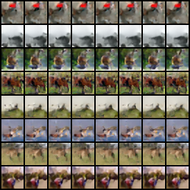
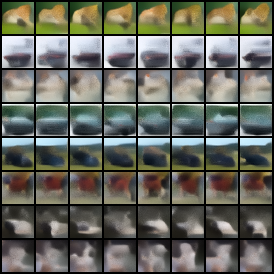
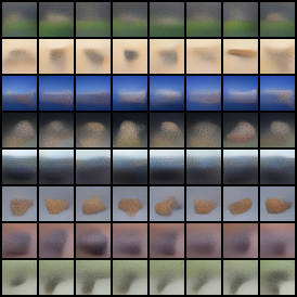
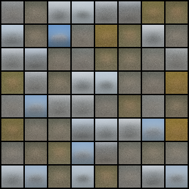
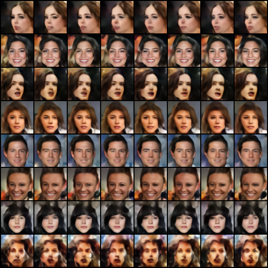
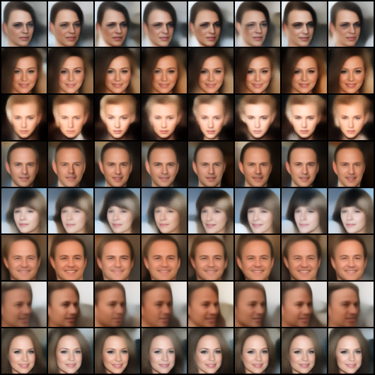
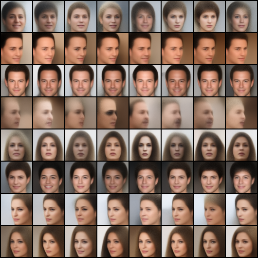
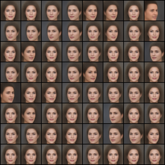
Here we try to visualize the representations learned by individual layers. We can get a rough idea of what's going on at layer i as follows:
-
Sample latent variables from all layers above layer i (Eq. 1).
-
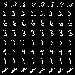
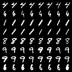
With these variables fixed, take S conditional samples at layer i (Eq. 2). Note that they are all conditioned on the same samples. These correspond to one row in the images below.
-
For each of these samples (each small image in the images below), pick the mode/mean of the conditional distribution of each layer below (Eq. 3).
-
Finally, sample an image x given the latent variables (Eq. 4).
Formally:
where s = 1, ..., S denotes the sample index.
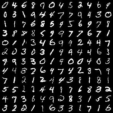
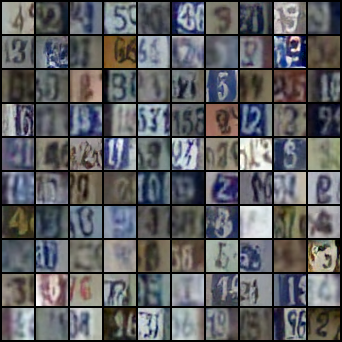
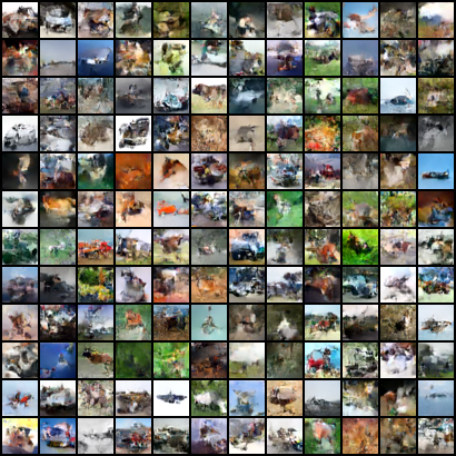
The equations above yield S sample images conditioned on the same values of z for layers i+1 to L. These S samples are shown in one row of the images below. Notice that samples from each row are almost identical when the variability comes from a low-level layer, as such layers mostly model local structure and details. Higher layers on the other hand model global structure, and we observe more and more variability in each row as we move to higher layers. When the sampling happens in the top layer (i = L), all samples are completely independent, even within a row.
I did not perform an extensive hyperparameter search, but this worked pretty well:
- Downsampling by a factor of 2 in the beginning of inference. After that, activations are downsampled 4 times for 64x64 images (CelebA and multi-dSprites), and 3 times otherwise. The spatial size of the final feature map is always 2x2. Between these downsampling steps there is approximately the same number of stochastic layers.
- 4 residual blocks between stochastic layers. Haven't tried with more than 4 though, as models become quite big and we get diminishing returns.
- The deterministic parts of bottom-up and top-down architecture are (almost) perfectly mirrored for simplicity.
- Stochastic layers have spatial random variables, and the number of rvs per "location" (i.e. number of channels of the feature map after sampling from a layer) is 32 in all layers.
- All other feature maps in deterministic paths have 64 channels.
- Skip connections in the generative model (
--skip). - Gated residual blocks (
--gated). - Learned prior of the top layer (
--learn-top-prior). - A form of data-dependent initialization of weights (
--data-dep-init). See code for details. - freebits=1.0 in experiments with more than 6 stochastic layers, and 0.5 for smaller models.
- For everything else, see
_add_args()inexperiment/experiment_manager.py.
With these settings, the number of parameters is roughly 1M per stochastic layer. I tried to control for this by experimenting e.g. with half the number of layers but twice the number of residual blocks, but it looks like the number of stochastic layers is what matters the most.
[1] CK Sønderby, T Raiko, L Maaløe, SK Sønderby, O Winther. Ladder Variational Autoencoders, NIPS 2016
[2] L Maaløe, M Fraccaro, V Liévin, O Winther. BIVA: A Very Deep Hierarchy of Latent Variables for Generative Modeling, NeurIPS 2019
[3] DP Kingma, T Salimans, R Jozefowicz, X Chen, I Sutskever, M Welling. Improved Variational Inference with Inverse Autoregressive Flow, NIPS 2016
[4] I Higgins, L Matthey, A Pal, C Burgess, X Glorot, M Botvinick, S Mohamed, A Lerchner. beta-VAE: Learning Basic Visual Concepts with a Constrained Variational Framework, ICLR 2017
[5] Y Burda, RB Grosse, R Salakhutdinov. Importance Weighted Autoencoders, ICLR 2016
[6] T Salimans, A Karpathy, X Chen, DP Kingma. PixelCNN++: Improving the PixelCNN with Discretized Logistic Mixture Likelihood and Other Modifications, ICLR 2017
[7] H Larochelle, I Murray. The neural autoregressive distribution estimator, AISTATS 2011
