utorch
utorch is a minimal implementation of pytorch and autograd. The idea was to create an understandable version of the deep learning framework, which means its code should be easy to follow even for someone who has no prior existence in machine learning, thus making it perfect for educators. To fulfill this requirement utorch supports the following features:
- simplegrad - automatic differentiation library that supports some predefined differentiable tensor operations
- neural network - a set of tools that allows to build and train neural networks. Those tools mimic the interface of PyTorch, so if you are familiar with PyTorch, then you are ready to go with utorch as well.
- utils - this library contains a set of tools that can be used to visualize the computational graphs.
Features that are intentionally not supported:
- GPU/TPU support. We would like to reduce the complexity of the code, providing python only implementation. Thus, we don't want to contaminate the code by adding c++ classes. However, if you have an idea on how to add this feature without changing the philosophy of this library please let us know.
nets
Nets package is a collections of tools based on simplegrad that allows to build and train neural networks.
Example 1: sklearn.datasets.make_classification
The first example is dedicated to solve a random n-class classification problem using a sklearn dummy dataset, see example 1.
In order to train the model you have to create the following components:
- Dataset. This can be done by creating an instance of Dataset
def build_dataset(config):
   train_x, train_y = datasets.make_classification(n_features=config["n_features"],
                                                   n_samples=config["n_samples"],
                                                   n_redundant=0,
                                                   n_classes=config["n_classes"])
   train_y = train_y.astype(int)
return DataLoader(train_x, train_y, config["batch_size"])- Model. An instance of class that inherits from Model. To make your life easier utorch provide a number of layers that you can use, see Model In this example, we will build a fully connected neural network model that contains of 2 hidden layers
class FullyConnected2NN(Model):
    def __init__(self, param_dict):
        self.layers = StackedLayers([
            LinearLayer(n_input=param_dict["n_input"], n_hidden=param_dict["n_hidden_1"], has_bias=param_dict["bias"],
                        name="input_layer"),
            ReLULayer(),
            LinearLayer(n_input=param_dict["n_hidden_1"], n_hidden=param_dict["n_hidden_2"],
                        has_bias=param_dict["bias"], name="hidden_layer_1"),
            ReLULayer(),
            LinearLayer(n_input=param_dict["n_hidden_2"], n_hidden=param_dict["n_class"], has_bias=False,
                        name="hidden_layer_2"),
        ]
        )

    def forward(self, x, *args, **kwargs):
return self.layers(x)-
loss. This entity is created to calculate the classification loss. You can use one of the losses that was prepared by us, see losses For the purpose of this exercises we will use CrossEntropyWithLogitsLoss
-
optimizer. You need to create an instance of Optimizer to train the model ;), see all avialable options in optim
-
train loop. This utility allows you to combine previously mentioned components into fully functional DL pipeline.
def train_model(model, criterion, optimizer, run_hist, data_loader, num_epochs=10):
    for epoch in range(num_epochs):
        for iteration, batch in enumerate(data_loader):
            inputs, labels = batch
            outputs = model(inputs)
            loss = criterion(outputs,  labels)
            optimizer.zero_grad()
            loss.backward()
            optimizer.update_model()

            run_hist["loss"].append(loss.value)

            print("epoch {},  it  {}, loss {} ".format(epoch, iteration, loss.value))
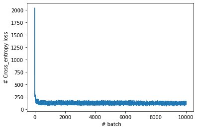
You can monitor training progress by visualizing learning curve:
and finally, we can calculate classification accuracy
def accuracy(prediction, target):
 values = np.argmax(prediction.value,axis=1)
 correct = np.sum(np.where(values == target, 1, 0))
 return correct/values.shape[0]

pred =  model(Variable(train_x))
accuracy(pred, target)
# out: ->  0.907140625
simplegrad
simplegrad is a tool that allows to generate computational graphs and automatically differentiate native Python and Numpy code. It can handle a large subset of Python's features, including loops, ifs, and recursion. In the future, it will take derivatives of derivatives of derivatives. It supports reverse-mode differentiation (a.k.a. backpropagation), which means it can efficiently take gradients of scalar-valued functions with respect to array-valued arguments.
If you are interested in the theory behind reverse-mode auto differentiation please take some time to read this remarkable phd thesis.
TODO add a tutorial on how the simplegrad is implemented.
Examples:
Dynamic computational graphs generation
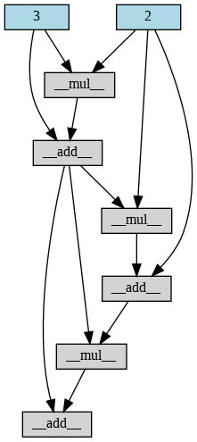
simplegrad allows creating a computational graph that represents all processing specified by a given python code, regardles on how complex it can be.
a =  Variable(2)
b = Variable(3)
for i in range(3):
  if i%2 == 0:
    b += a*b
  else:
    a += a*b
draw_graph(b)
and something a little bit more complicated
def fib(n):
  if n == 0 or n ==1:
    return n
  return fib(n-1)+fib(n-2)

n = Variable(10)
b = fib(n)
Automatic derivative calculation
The main purpose of this package is the ability to calculate the derivative of the scalar input with respect to the n-dim vector input. In the literature, it is called reverse-mode differentiation. A more detailed explanation of this idea will be added soon. In the meantime, for more information, please refer to this paper.
From the user perspective, in order to calculate derivative one need to cal the method backward(), see examples below. To make sure, that the simplegrad returns the correnct answer, we compare it with the one given by PyTorch.
Example 1: Simple expression composed of sums and multiplications
a =  Variable(2)
b = Variable(3)
d = Variable(4)
c = a*a*b+d+d*a*b+a*a*2
c.backward()
print(a.grad.value, b.grad.value, d.grad.value)
(32, 12, 7)
A = torch.tensor(2., requires_grad=True)
B = torch.tensor(3.,requires_grad=True)
D = torch.tensor(4.,requires_grad=True)
C = A*A*B+D+D*A*B+A*A*2


C.backward()
print(A.grad, B.grad, D.grad)
Example 2: 2D tensor manipulation:
# simplegrad implementation
np.random.seed(10)
d = Variable(np.random.normal(1,10,size=(2,3)))
w = Variable(np.random.normal(1,10,size=(10,3)))
b = Variable(np.random.normal(1,10,size=(10)))
c = Variable.sum(d@Variable.transpose(w)*b)

c.backward()
print("d grad ",d.grad.shape(), d.grad.value,)
print("w grad ",w.grad.shape(), w.grad.value,)
print("b grad ",b.grad.shape(), b.grad.value,)
draw_graph(c)
d grad (2, 3) [[-115.06495011 6.3034526 -265.32755501]
[-115.06495011 6.3034526 -265.32755501]]
w grad (10, 3) [[ 76.19211818 76.86301452 -103.31766542]
[ -36.19622066 -36.51494014 49.08262304]
[ 206.61821525 208.43755574 -280.17742705]
[ -96.26176228 -97.10937836 130.53240658]
[ 115.79867166 116.81831658 -157.02475139]
[ -38.21287309 -38.54934985 51.81723426]
[-127.86271216 -128.98858487 173.3837729 ]
[ -59.30394821 -59.82613874 80.41705135]
[-107.3235098 -108.26852816 145.53230364]
[ -17.16613424 -17.31728763 23.27753784]]
b grad (10,) [ 66.17945244 -198.59804888 -26.2728396 -124.81752913 478.64093321
-707.33450232 417.64276678 54.54966854 -142.59286261 98.19945202]
#pytorch implementation
np.random.seed(10)
D = torch.tensor(np.random.normal(1,10,size=(2,3)), requires_grad=True)
W = torch.tensor(np.random.normal(1,10,size=(10,3)), requires_grad=True)
B = torch.tensor(np.random.normal(1,10,size=(10)),requires_grad=True)

C = torch.sum(D@W.T*B)

C.backward()

print("d grad ",D.grad.shape, D.grad,)
print("w grad ",W.grad.shape, W.grad,)
print("B grad ",B.grad.shape, B.grad,)
d grad torch.Size([2, 3]) tensor([[-115.0650, 6.3035, -265.3276],
[-115.0650, 6.3035, -265.3276]], dtype=torch.float64)
w grad torch.Size([10, 3]) tensor([[ 76.1921, 76.8630, -103.3177],
[ -36.1962, -36.5149, 49.0826],
[ 206.6182, 208.4376, -280.1774],
[ -96.2618, -97.1094, 130.5324],
[ 115.7987, 116.8183, -157.0248],
[ -38.2129, -38.5493, 51.8172],
[-127.8627, -128.9886, 173.3838],
[ -59.3039, -59.8261, 80.4171],
[-107.3235, -108.2685, 145.5323],
[ -17.1661, -17.3173, 23.2775]], dtype=torch.float64)
B grad torch.Size([10]) tensor([ 66.1795, -198.5980, -26.2728, -124.8175, 478.6409, -707.3345,
417.6428, 54.5497, -142.5929, 98.1995], dtype=torch.float64)
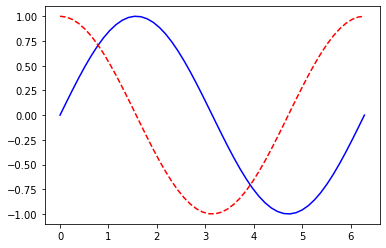
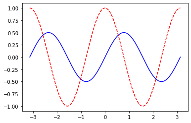
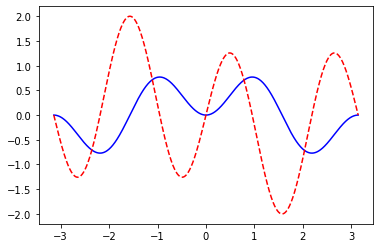
Visualize 1D function and its 1st derivative:
def plot_function_and_der(fun, range=[0,1], n_points=100):

  def evaluate_derivative(x, fun):
    x_var = Variable(x)
    y = fun(x_var)
    y.backward()
    return y.value, x_var.grad.value

  x_points = np.linspace(start = range[0], stop=range[1], num=n_points)
  y = np.transpose(np.array(list(map(lambda x: evaluate_derivative(x, fun), x_points))))
  plt.plot(x_points, y[0], color='blue')
  plt.plot(x_points, y[1], color='red', linestyle='dashed')
plot_function_and_der( Variable.sin, range=[0,2*np.pi], n_points=50)
plot_function_and_dev(lambda x: Variable.sin(x)*Variable.cos(x), range=[-np.pi,np.pi], n_points=1000)
plot_function_and_dev(lambda x: Variable.sin(x)*Variable.sin(x*2), range=[-np.pi,np.pi], n_points=1000)
Contribution
You are more than welcome to contribute to this software. If you plan to contribute new features, utility functions, or extensions to the core, please first open an issue and discuss the feature with us. Please keep in mind the purpose of this software is to provide understandable implementation of the Deep Learning framework. We don't want to compete with pytorch, jax or tensorflow. Our goal is to give students and ML practitioners source code that they can leverage to get a better feeling on how general DL framework works.
Citation
@software{utorch,
  author = {Adam Dendek},
  title = {{utorch}: a minimal implementation of autograd and pytorch},
  url = {https://github.com/adendek/utorch},
  version = {0.1},
  year = {2021},
}
