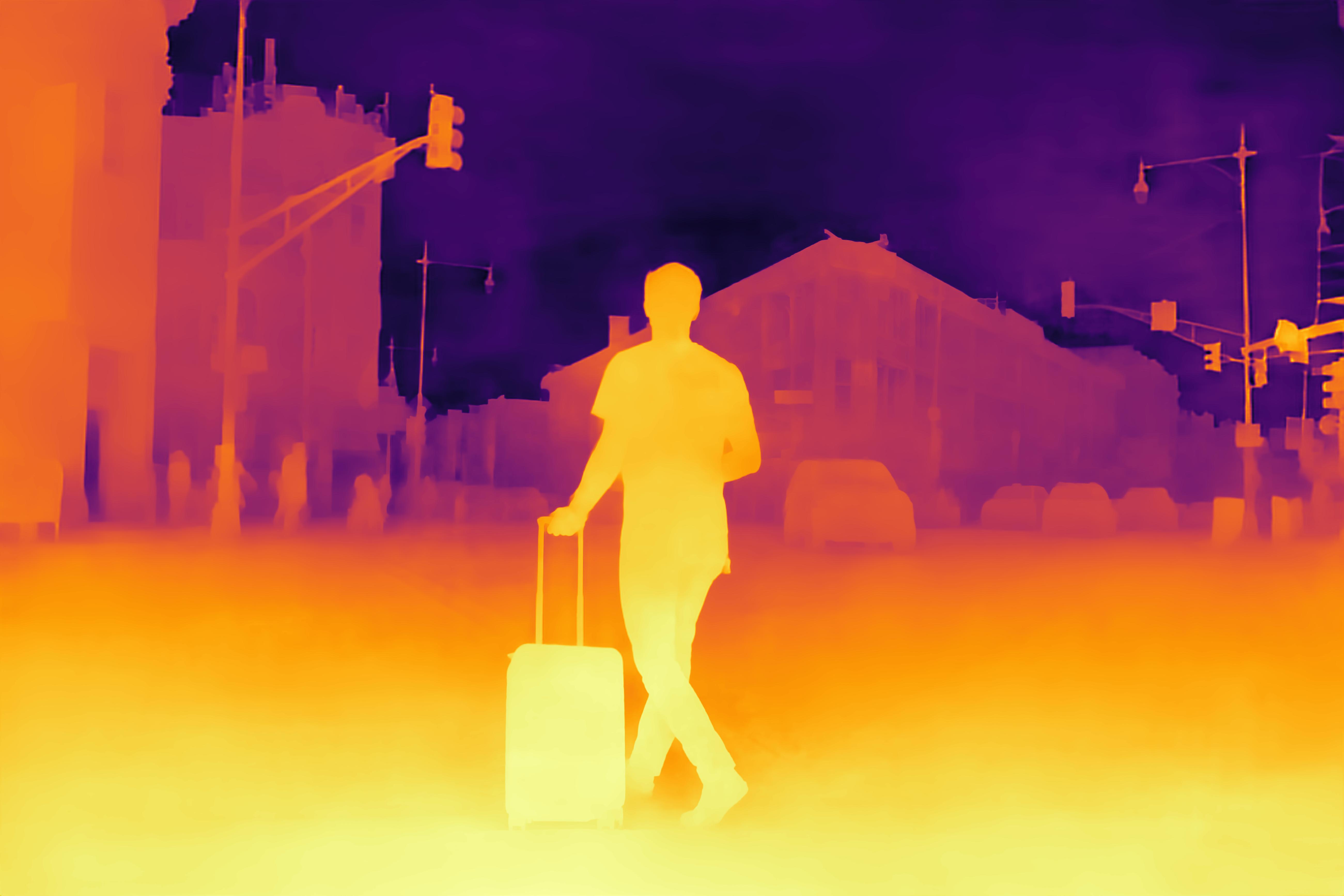
(NEW!) LeRes is now supported within our method.
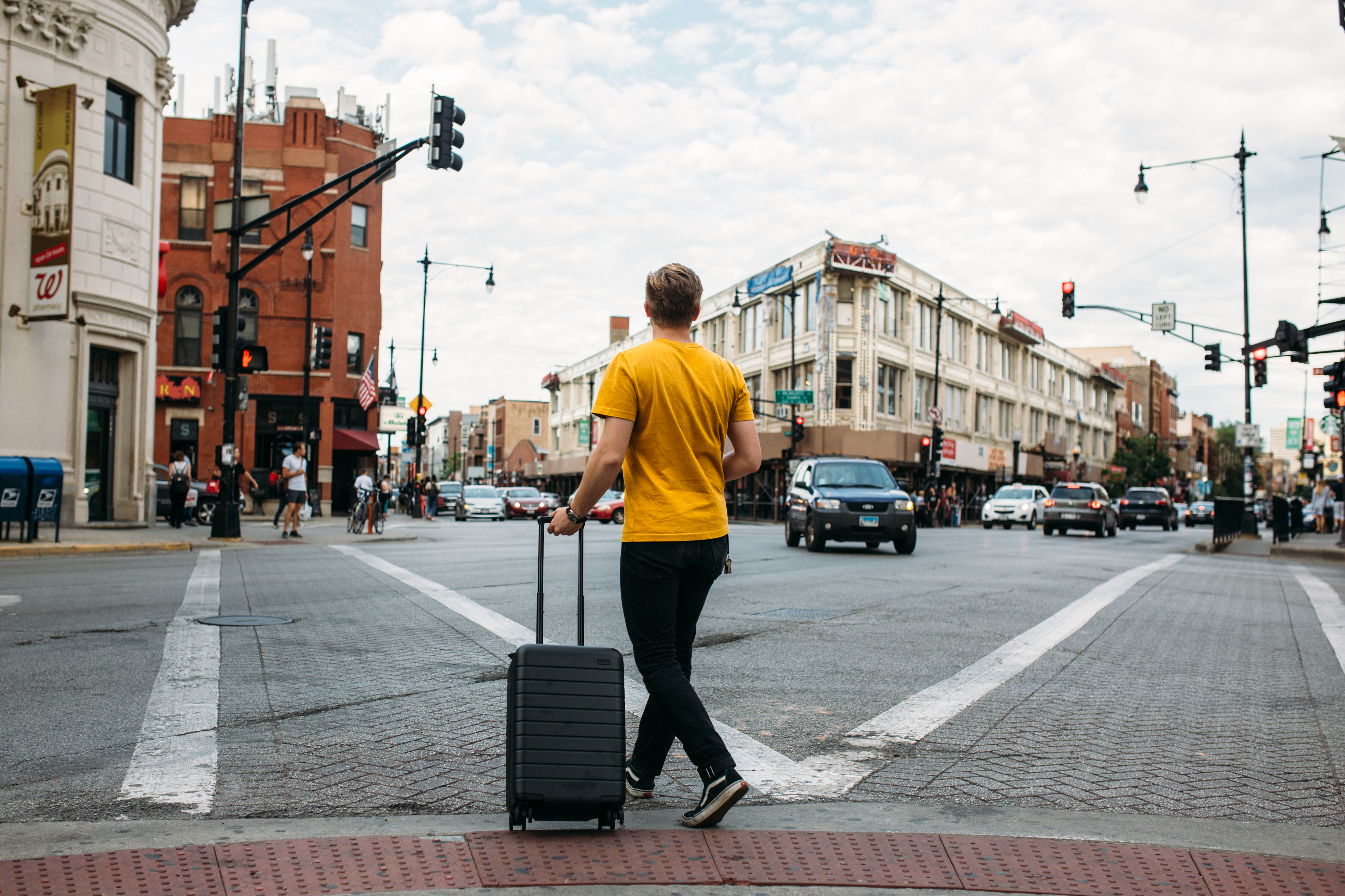
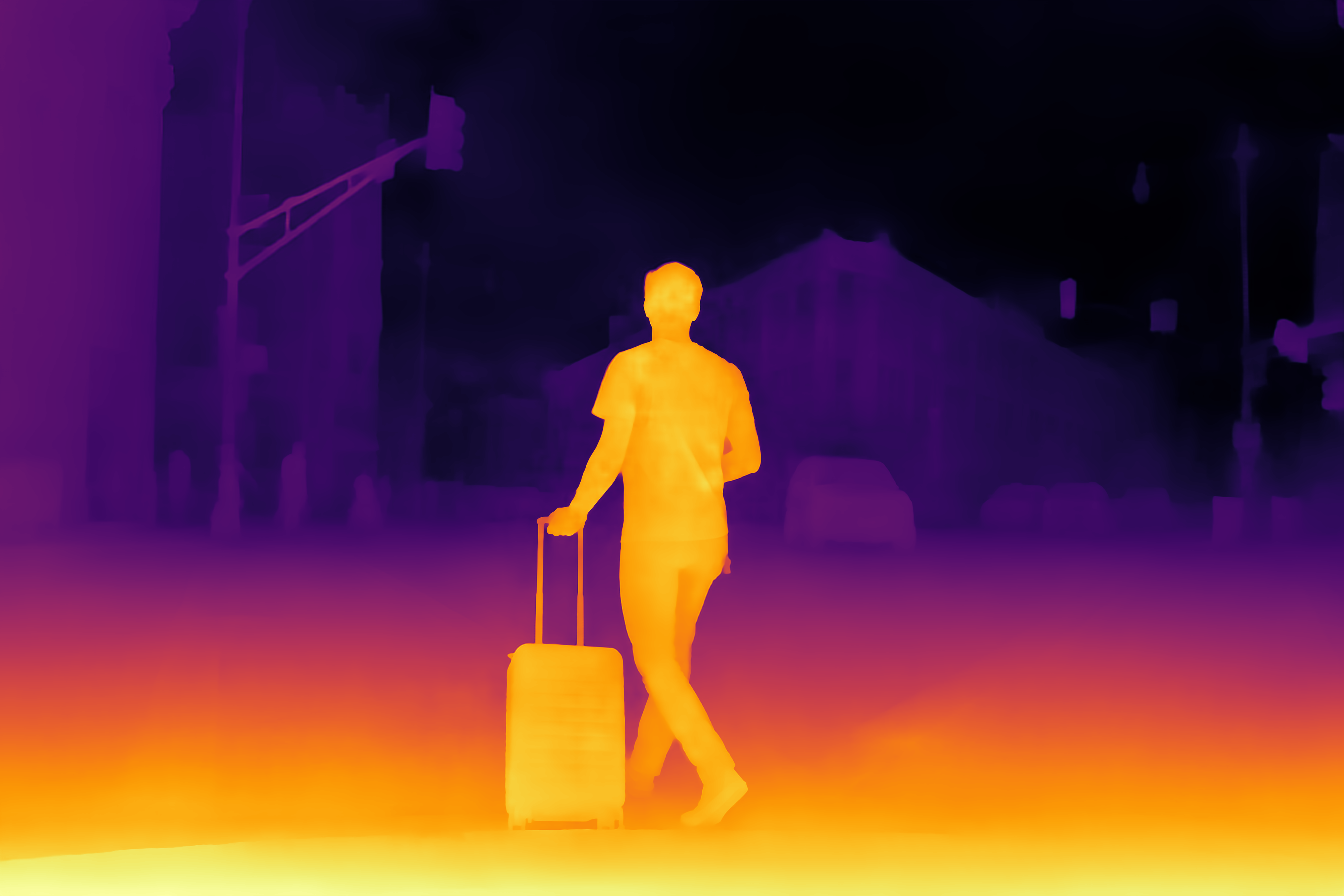
Here is a visualization of the improvement gained using LeRes instead of MiDas.
| RGB | Our method using MiDaS | Our method using LeRes (NEW!) |
|---|---|---|
 |
 |
 |
Use --max_res as input argument for run.py in combination with --Final to set a limit on the resolution of the results that our method generates.
We provide this parameter as a trade-off between run-time and resolution. Using this reduces the run-time if only a result up to specific-megapixel is needed.
This parameter sets a limit on the bigger dimension of the result in term of pixels (while keeping aspect ratio). For example, to generate results with a bigger dimension size up to 2000 pixels use the following:
python run.py --Final --max_res 2000 --data_dir PATH_TO_INPUT --output_dir PATH_TO_RESULT --depthNet 0Boosting Monocular Depth Estimation Models to High-Resolution via Content-Adaptive Multi-Resolution Merging
S. Mahdi H. Miangoleh*, Sebastian Dille*, Long Mai, Sylvain Paris, Yağız Aksoy. Main pdf, Supplementary pdf, Project Page.
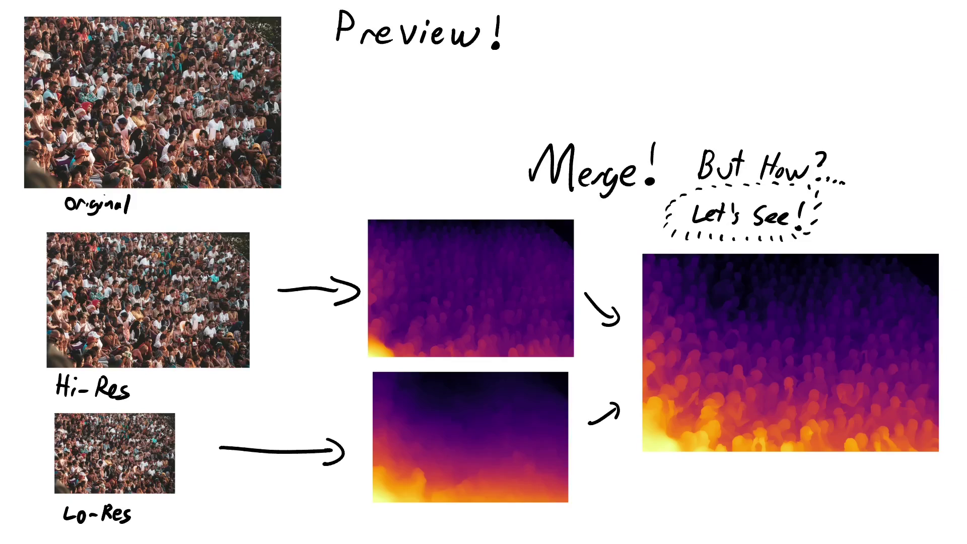
We propose a method that can generate highly detailed high-resolution depth estimations from a single image. Our method is based on optimizing the performance of a pre-trained network by merging estimations in different resolutions and different patches to generate a high-resolution estimate.
Try our model easily on Colab :
- (NEW!) Now you can set the maximum resolution of the results to reduce runtime.
- (NEW!) Our method implementation using LeReS is now available. [July 2021]
- A Quick overview of the method is now presented in README.md. [July 2021]
- Google Colaboratory notebook is now available. [June 2021]
- Merge net training dataset generation instructions is now available. [June 2021]
- Bug fix. [June 2021, July 2021]
We use existing monocular depth estimation networks to generate highly detailed estimations without re-training.
We achieve our results by getting several estimations at different resolutions. We then merge these into a structurally consistent high-resolution depth map followed by a local boosting to enhance the results and generate our final result.
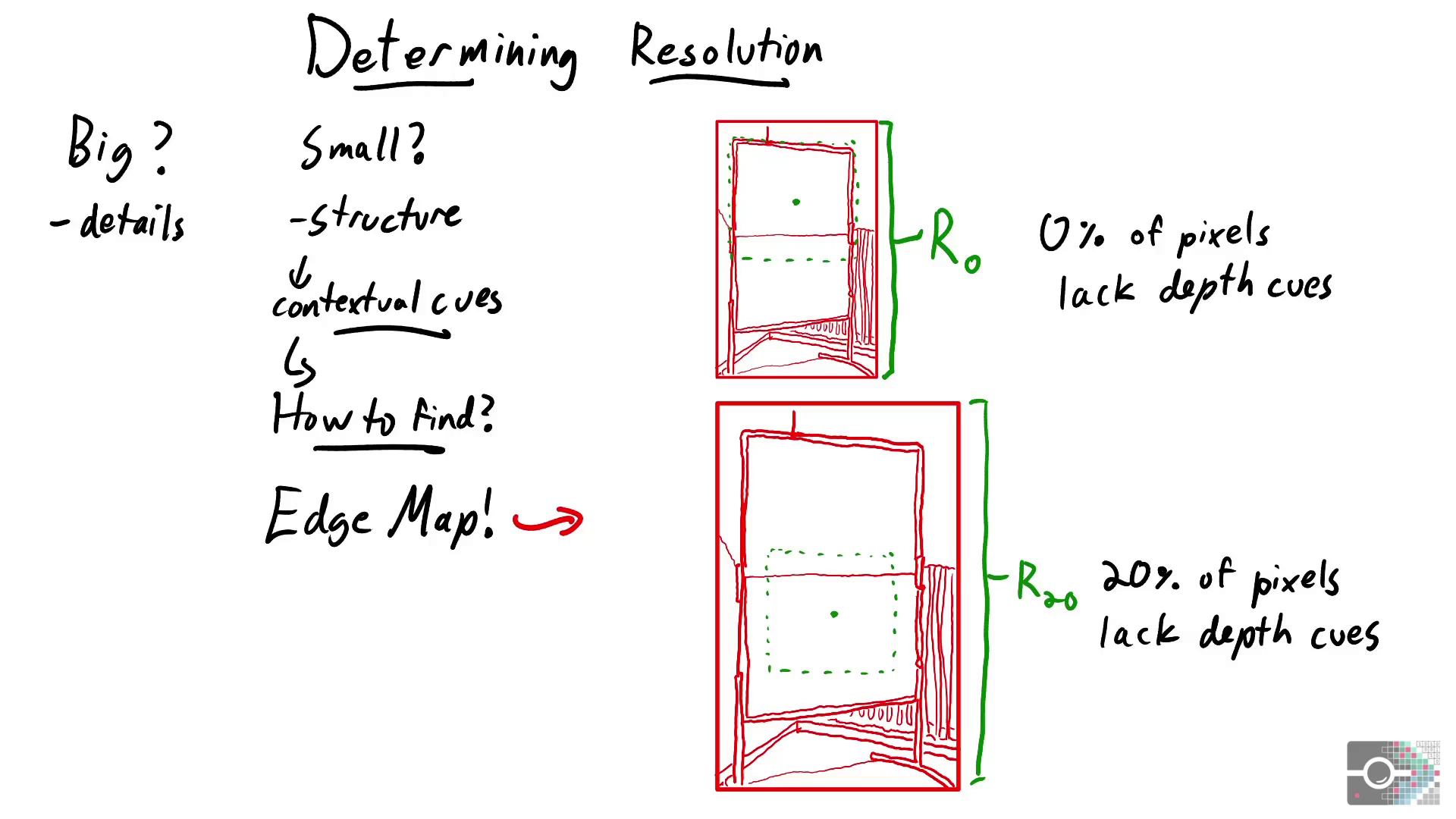
Monocular depth estimation uses contextual cues such as occlusions or the relative sizes of objects to estimate the structure of the scene.
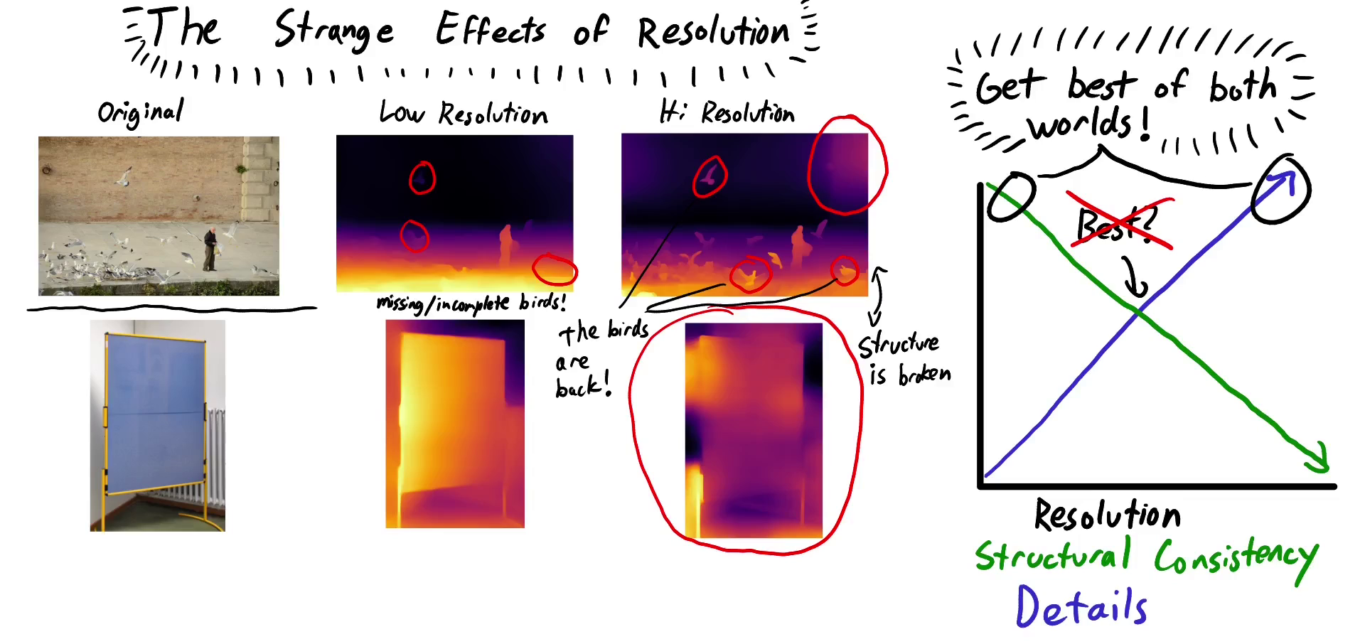
We will use a pre-trained MiDas-v2 here, but our analysis with the SGR network also supports our claims.
When we feed the image to the network at different resolutions, some interesting patterns arise. At lower resolutions, many details in the scene are missing, such as birds in this example. At high resolutions, however, we start to see inconsistent overall structure, and this flat board gets significantly less flat. The advantage is that the network is able to generate high frequency details. This shows that there is a trade-off between structural consistency and high-frequency details with respect to input resolution.
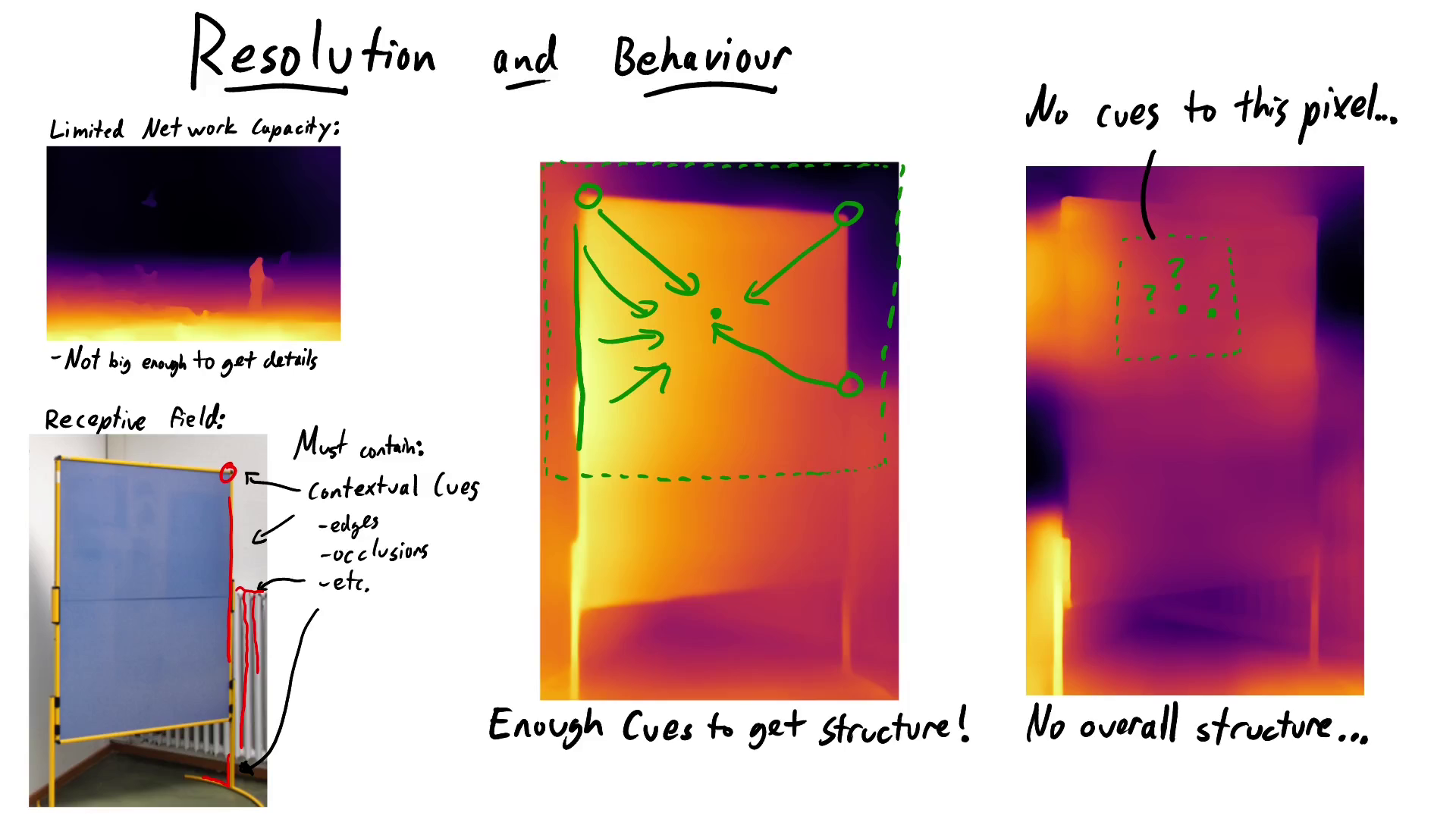
We explain this behavior through two properties of convolutional neural networks: limited receptive field size and network capacity. The lack of high frequency details in low resolutions are due to a limited network capacity. A small network that generates the structure of a complex scene cannot also generate fine details.
The loss of structure at high resolutions comes from a limited receptive field size. The receptive field is the region around a pixel that contributes to the estimation at that pixel. It is set by the network configuration and training resolution, and effectively gets smaller as resolution increases. At a low resolution, every pixel can see the edges of the board, so the network judges that this is a flat wall. At a high resolution, however, some pixels do not receive any contextual information. This results in large structural inconsistencies.
For any given image, we determine the highest resolution that will result in a consistent structure by making sure that every pixel has contextual information. For this purpose, we need the distribution of contextual cues in the image. We approximate contextual cues with a simple edge map.
The resolution where every pixel is at most a half receptive field size away from context edges is called R_0. When we increase the resolution any further, structural inconsistencies will arise but more details will be generated. When 20% of the pixels do not receive any context, we call this resolution R_20. Note that R_0 and R_20 depend on the image content!
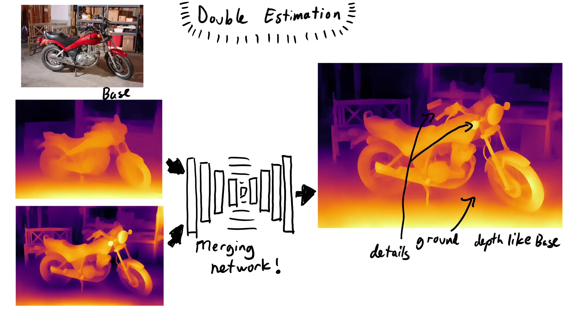
We are still able to go beyond R0 by merging the high-frequency details in the R20 resolution onto the structure of the base resolution. We call this Double Estimation. We train an image-to-image translation network to merge the low-resolution depth range of the base with the high-resolution details of R_20. It does so without inheriting the structural inconsistencies of the high-res input. This way, we go beyond R_0 and generate more details by using R_20 as our high-resolution input. In fact, the network is so robust against low-frequency artifacts that we can even use R_20 as our high-resolution input.
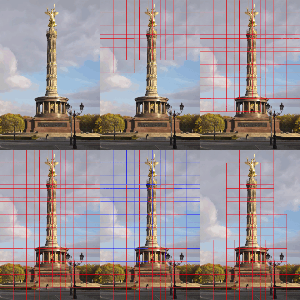
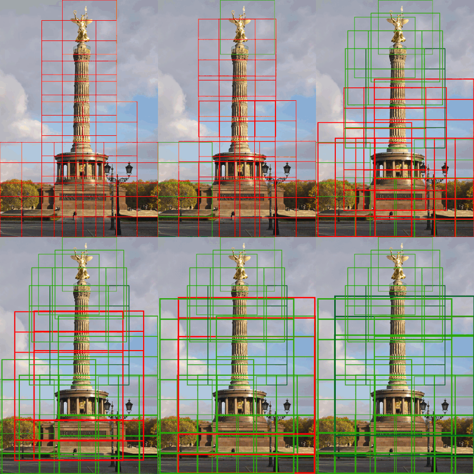
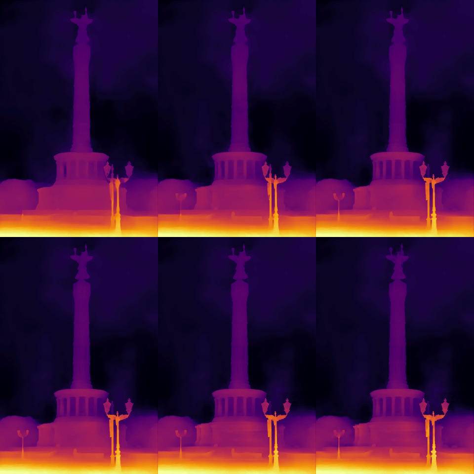
Note that R20 is bounded by the smoothest regions in the image, while there are image patches that could support a higher resolution. We choose candidate patches by tiling the image and discarding all patches without useful details (step1). The leftover patches are expanded until their edge density matches that of the image(step2). Finally, we merge a double estimation for each patch onto our R20 results and generate our final results (step3).
| Step 1: Tile and discard | Step 2: Expand | Step 3: Merge |
|---|---|---|
 |
 |
 |
We Provided the implementation of our method using MiDas-v2, LeReS and SGRnet as the base. Note that MiDas-v2 and SGRnet estimate inverse depth while LeReS estimates depth.
Our mergenet model is trained using torch 0.4.1 and python 3.7 and is tested with torch<=1.8.
Download our mergenet model weights from here and put it in
.\pix2pix\checkpoints\mergemodel\latest_net_G.pth
To use MiDas-v2 or LeReS as base: Install dependancies as following:
conda install pytorch torchvision opencv cudatoolkit=10.2 -c pytorch
conda install matplotlib
conda install scipy
conda install scikit-image
For MiDaS-v2, download the model weights from MiDas-v2 and put it in
./midas/model.pt
activate the environment
python run.py --Final --data_dir PATH_TO_INPUT --output_dir PATH_TO_RESULT --depthNet 0
For LeReS, download the model weights from LeReS (Resnext101) and put it in root:
./res101.pth
activate the environment
python run.py --Final --data_dir PATH_TO_INPUT --output_dir PATH_TO_RESULT --depthNet 2
To use SGRnet as base: Install dependencies as following:
conda install pytorch=0.4.1 cuda92 -c pytorch
conda install torchvision
conda install matplotlib
conda install scikit-image
pip install opencv-python
Follow the official SGRnet repository to compile the syncbn module in ./structuredrl/models/syncbn. Download the model weights from SGRnet and put it in
./structuredrl/model.pth.tar
activate the environment
python run.py --Final --data_dir PATH_TO_INPUT --output_dir PATH_TO_RESULT --depthNet 1
Different input arguments can be used to generate R0 and R20 results as discussed in the paper.
python run.py --R0 --data_dir PATH_TO_INPUT --output_dir PATH_TO_RESULT --depthNet #[0,1 or 2]
python run.py --R20 --data_dir PATH_TO_INPUT --output_dir PATH_TO_RESULT --depthNet #[0,1 or 2]
To generate the results with CV.INFERNO colormap use --colorize_results like the sample below:
python run.py --colorize_results --Final --data_dir PATH_TO_INPUT --output_dir PATH_TO_RESULT --depthNet #[0,1 or 2]Fill in the needed variables in the following matlab file and run:
./evaluation/evaluatedataset.m
- estimation_path : path to estimated disparity maps
- gt_depth_path : path to gt depth/disparity maps
- dataset_disp_gttype : (true) if ground truth data is disparity and (false) if gt depth data is depth.
- evaluation_matfile_save_dir : directory to save the evalution results as .mat file.
- superpixel_scale : scale parameter to run the superpixels on scaled version of the ground truth images to accelarate the evaluation. use 1 for small gt images.
Navigate to dataset preparation instructions to download and prepare the training dataset.
python ./pix2pix/train.py --dataroot DATASETDIR --name mergemodeltrain --model pix2pix4depth --no_flip --no_dropoutpython ./pix2pix/test.py --dataroot DATASETDIR --name mergemodeleval --model pix2pix4depth --no_flip --no_dropoutThis implementation is provided for academic use only. Please cite our paper if you use this code or any of the models.
@INPROCEEDINGS{Miangoleh2021Boosting,
author={S. Mahdi H. Miangoleh and Sebastian Dille and Long Mai and Sylvain Paris and Ya\u{g}{\i}z Aksoy},
title={Boosting Monocular Depth Estimation Models to High-Resolution via Content-Adaptive Multi-Resolution Merging},
journal={Proc. CVPR},
year={2021},
}
The "Merge model" code skeleton (./pix2pix folder) was adapted from the pytorch-CycleGAN-and-pix2pix repository.
For MiDaS, LeReS and SGR inferences we used the scripts and models from MiDas-v2, LeReS and SGRnet respectively (./midas, ./lib and ./structuredrl folders).
Thanks to k-washi for providing us with a Google Colaboratory notebook implementation.
