One of the fundamental challenges in the field of image processing and computer vision is image denoising, where the underlying goal is to estimate the original image by suppressing noise from a noise-contaminated version of the image. Image noise may be caused by different intrinsic (i.e., sensor) and extrinsic (i.e.environment) conditions which are often not possible to avoid in practical situations. Therefore, image denoising plays an important role in a wide range of applications such as image restoration, visual tracking, image registration, image segmentation, and image classification, where obtaining the original image content is crucial for strong performance. While many algorithms have been proposed for the purpose of image denoising, the problem of image noise suppression remains an open challenge, especially in situations where the images are acquired under poor conditions where the noise level is very high. We will be exploring non-local means algorithm for image denoising in this repository.
The NLM is a greedy algorithm. We convert the image into a matrix with their color values (in this case gray-scale values). The basic idea to denoise an image is to do some sort of averaging and restoration of the image. Since considering only a single pixel value is error prone, we zoom out a bit to consider a small square around the pixel of interest. This small square is called a patch. A patch is transformed into a feature vector simply by reshaping it as a vector. It can also be interpreted as the coordinates of the central pixel in a high dimensional space that describes all the possible image patches. Then the distance between similar patches is computed. The denoised value of a given pixel is obtained as the weighted average of the other pixels of the image, where the weight (or contribution) of each pixel is inversely proportional to the distance between its patch and the reference patch of the pixel to denoise. Since the above process is computationally of very large running time, we limit the similarity search area to a window around the patch. This, in a way, does limit the non-locality of the algorithm, but makes it practically possible to use.
The following is the stepwise procedure followed for running NLM denoising algorithm on the image:
-
The image is padded using reflect mode( adding extra boundary around image using the color values already present in the image) to create a wrap around boundary. This step ensures that we don't go out of bounds while finding window and neighbours around particles near the image boundary
-
After padding the image, the small window surrounding each pixel is precomputed and stored in a 4D matrix to reduce the running complexity. Later, the pixels in the small window around any pixel can be found just by indexing the 4D array properly.
-
Essentially, the algorithm modifies each pixel value by a weighted average of all the other pixels, and the weight values are determined by neighborhood similarity using the formulas given in the research paper. For each pixel and patch, similar patches are found in the search window, and their weighted averages are taken. The search window is limited to some value to reduce the running time of the algorithm as explained above.
-
Small window: It is related to the patch size when comparing similar neighborhoods. We can't choose a very big patch because all patches will be different. We cannot choose a small patch either, otherwise all patches will be similar. Therefore, here we take the small window size to be 7.
-
Big window: It is related to the big neighborhood to search for patches as explained above. The bigger the window the better will be the non-local results, but it will have larger computational needs. So, considering optimal tradeoff between CPU and accuracy, here we choose Big Window to be 21
-
Sigma h: It is the constant used to control patch difference when we calculate the weights between patches. It is also closely related to the noise variance present on image, and it may depend from pixel to pixel. This parameter will vary from image to image
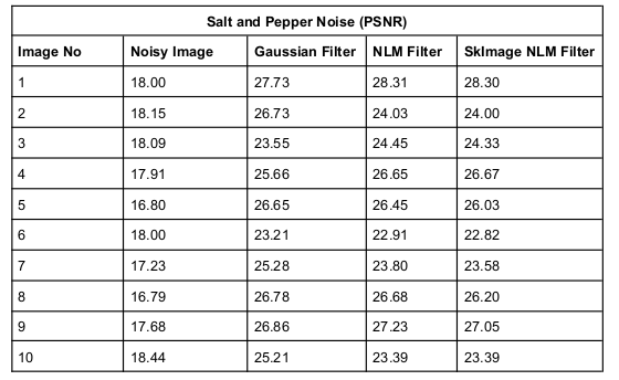
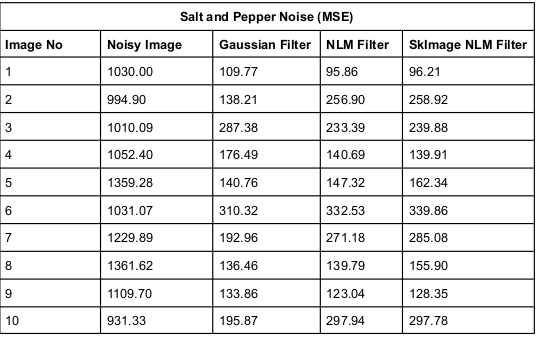
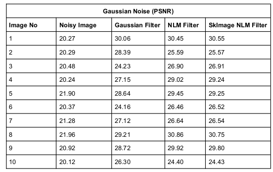
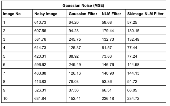
Metrics (MSE and PSNR) obtained for both gaussian filtering, NLM filtering, SkImage NLM filtering and the noisy image for all the 10 images, using some fixed h value (in this case 30)
Note: Better NLM values can be obtained using different salt_and_pepper_h value and gaussian_h_value. These tabulations only consider both h to be equal to 30.
| SNP Noise PSNR | SNP Noise MSE |
|---|---|
 |
 |
| Gaussian Noise PSNR | Gaussian Noise MSE |
|---|---|
 |
 |
The Gaussian filter blurs the noisy image, thus reducing the visual quality of the image whereas the NLM filter preserves the edges by finding similar patches in a non-local area and trying to eliminate the noise with better averaging. In some cases we can observe from the data and the result images, that gaussian filtering is better or comparable with the NLM filtering, both in metrics and visually. It is because the image is of better resolution (such as image 8) and thus the gaussian filtering blurring effect is not visible on the edges of the image.
It can be seen from the above data, that in most of the cases in salt and pepper noise, NLM filtering provides slightly better (almost comparable) results to gaussian filtering. In salt and pepper noise, the pixel values are deviating from the original value at specific random points. Therefore, the gaussian filter blurring effect averages out the pixel values from its immediate neighbours. Therefore the gaussian filtering method works comparable to NML for salt and pepper noises on metrics. However, if the image resolution is not good then visually NML image is much better than gaussian filtering.
In gaussian noise, we can see from the data that the NLM outperforms gaussian filtering in almost all the images both visually and on metrics. This is because the noise is distributed normally at random and thus the NLM patch similarity functionality restores the image much better than the blurring gaussian filter.
In general, the NLM filter works well in cases where there are large patches of the image with a similar color value, whereas the gaussian filtering does not usually preserve edges.
Note: Results for filters and noise can be found under the results directory in the repo. Nevertheless, the same can be again generated by running the code. Other images can be used as well
-
The dataset is being downloaded from the given hashed link. However if at a later point of time, the dataset is not available in the input file, kindly use the image dataset present in the repository in place of the downloaded data.
-
To run, open the python notebook file and select the image using the slider given. Then run the corresponding cells to get the results
- A. Buades, B. Coll and J. -. Morel, "A non-local algorithm for image denoising," 2005 IEEE Computer Society Conference on Computer Vision and Pattern Recognition (CVPR'05), San Diego, CA, USA, 2005, pp. 60-65 vol. 2, doi: 10.1109/CVPR.2005.38
- Palou, G. (2015, July 07). An approach to Non-Local-Means denoising. http://dsvision.github.io/an-approach-to-non-local-means-denoising.html Last Accessed 15 Aug 2021
- Angelo, Emmanuel. "Introducing NL-Means" 2020, http://www.computersdontsee.net/post/2013-02-09-introducing-nl-means/ Last Accessed 15 Aug 2021
- Angelo, Emmanuel. "NL-Means: Some Math" 2020, http://www.computersdontsee.net/post/2013-04-13-nl-means-some-math/ Last Accessed 15 Aug 2021
- Angelo, Emmanuel. "Implementing NL-Means" 2020, http://www.computersdontsee.net/post/2013-04-13-implementing-nl-meaans/ Last Accessed 15 Aug 2021