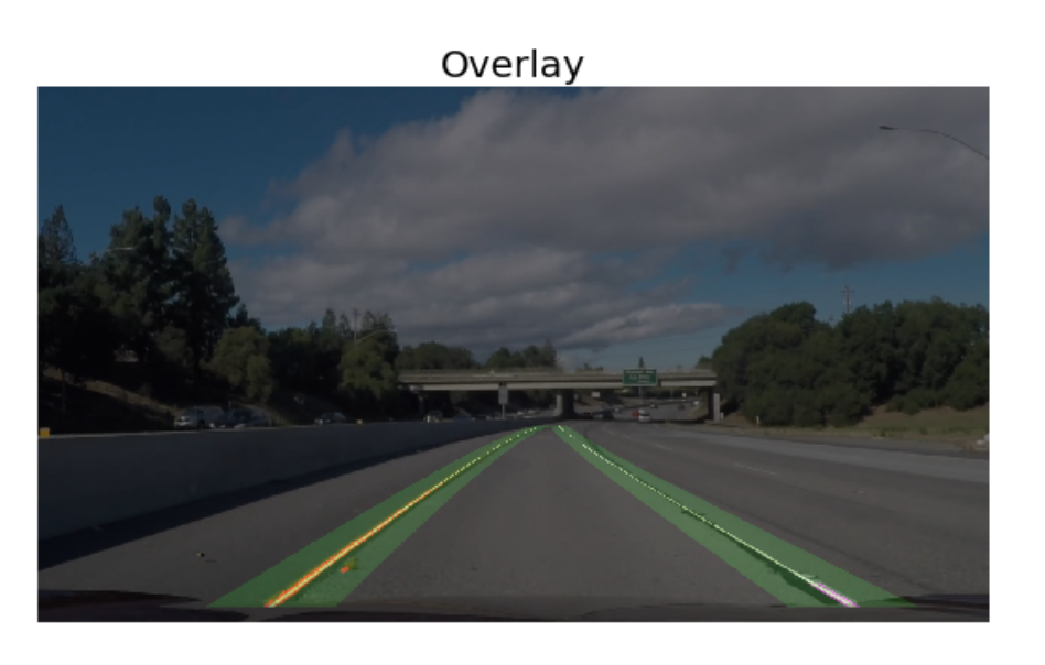
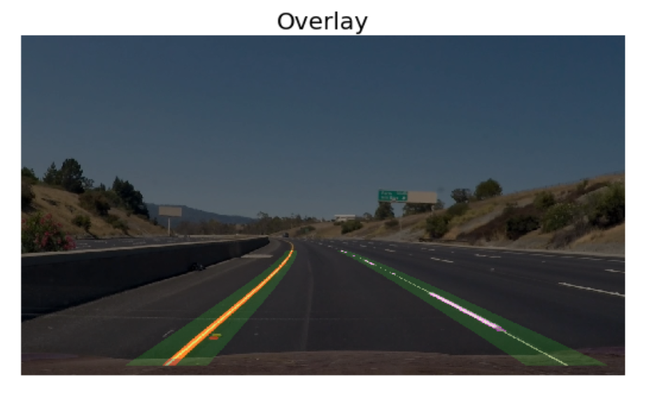
The goal of this project is to use traditional Computer Vision (i.e. non-machine learning)
techniques to develop an advanced and robust algorithm that can detect and track lane boundaries in a video.
The pipeline highlighted below was designed to operate under the following scenarios:
Assumptions:
- It can detect exactly two lane lines, i.e. the left and right lane boundaries of the lane the vehicle is currently driving in.
- It cannot detect adjacent lane lines
- The vehicle must be within a lane and must be aligned along the direction of the lane
- If only one of two lane lines have been successfully detected, then the detection is considered invalid and will be discarded. In this case, the pipeline will instead output a lane line fit (for both left and right) based on the moving average of the previous detections. This is due to the lack of an implementation of the lane approximation function (which is considered as future work).
- Python 3.x
- NumPy
- Matplotlib (for charting and visualising images)
- OpenCV 3.x
- Pickle (for storing the camera calibration matrix and distortion coefficients)
All the dependencies needed are in the requirements.txt file.
pip install requirements.txt
Tha camera Calibration matrix is already given in the dataset. #Camera Matrix K = [[ 1.15422732e+03 0.00000000e+00 6.71627794e+02] [ 0.00000000e+00 1.14818221e+03 3.86046312e+02] [ 0.00000000e+00 0.00000000e+00 1.00000000e+00]]
#Distortion Coefficients dist = [[ -2.42565104e-01 -4.77893070e-02 -1.31388084e-03 -8.79107779e-05 2.20573263e-02]]
The various steps involved in the pipeline are as follows, each of these has also been discussed in more detail in the sub sections below:
- Apply a distortion correction to raw images.
- Apply a perspective transform to rectify image ("birds-eye view").
- Use color transforms, gradients, etc., to create a thresholded binary image.
- Detect lane pixels and fit to find the lane boundary.
- Determine the curvature of the lane and vehicle position with respect to center.
- Warp the detected lane boundaries back onto the original image.
- Output visual display of the lane boundaries and numerical estimation of lane curvature and vehicle position.
Distortion occurs when the camera maps/transforms the 3D object points to 2D image points.
Since this transformation process is imperfect, the apparent shape/size/appearance of some of the
objects in the image change i.e. they get distorted. Since we are trying to accurately place the car in
the world, look at the curve of a lane and steer in the correct direction, we need to correct for this distortion. Otherwise, our measurements are going to be incorrect.
The first step of the entire process is undistorting the image. Since the image is taken by the camera it has various distortions in it. Such as radial distortion, spherical aberration etc. hence we need a calibration matrix to obtain a proper video frame. In an undistorted image, straight lines seem to curve slightly as we move away from the center of the image. This can cause unwanted results in the process further. Hence it is of utmost necessity to undistort the image.
- We undistort raw images by passing them into
cv2.undistortalong with the two params given above.
The second most important step in the process pipeline is denoising the image. We have used median filter to remove salt and pepper noise and have used gaussian filter as well. However, the difference isn’t that drastic and noticeable.
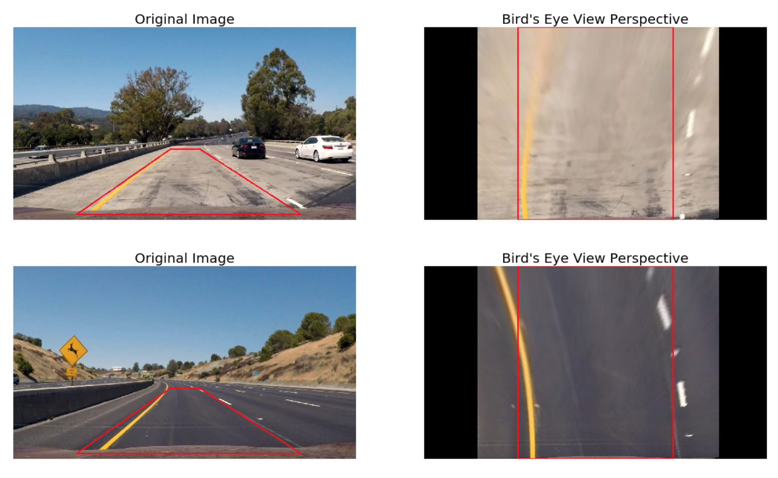
Following the distortion correction, an undistorted image undergoes Perspective Transformation which warpes the image into a bird's eye view scene. This makes it easier to detect the lane lines (since they are relatively parallel) and measure their curvature.
- Firstly, we compute the transformation matrix by passing the
srcanddstpoints intocv2.getPerspectiveTransform. These points are determined empirically with the help of the suite of test images. - Then, the undistorted image is warped by passing it into
cv2.warpPerspectivealong with the transformation matrix - Finally, we cut/crop out the sides of the image using a utility function
get_roi()since this portion of the image contains no relevant information
An example of this has been showcased below for convenience.
This was by far the most involved and challenging step of the pipeline. An overview of the test videos and a review of the U.S. government specifications for highway curvature revealed the following optical properties of lane lines (on US roads):
- Lane lines have one of two colours, white or yellow
- The surface on both sides of the lane lines has different brightness and/or saturation and a different hue than the line itself, and,
- Lane lines are not necessarily contiguous, so the algorithm needs to be able to identify individual line segments as belonging to the same lane line.
The latter property is addressed in the next two subsections whereas this subsection leverages the former two properties to develop a filtering process that takes an undistorted warped image and generates a thresholded binary image that only highlights the pixels that are likely to be part of the lane lines. Moreover, the thresholding/masking process needs to be robust enough to account for uneven road surfaces and most importantly non-uniform lighting conditions.
Many techniques such as gradient thresholding, thresholding over individual colour channels of different color spaces and a combination of them were experimented with over a training set of images with the aim of best filtering the lane line pixels from other pixels. The experimentation yielded the following key insights:
-
The performance of indvidual color channels varied in detecting the two colors (white and yellow) with some transforms significantly outperforming the others in detecting one color but showcasing poor performance when employed for detecting the other. Out of all the channels of RGB, HLS, HSV and LAB color spaces that were experiemented with the below mentioned provided the greatest signal-to-noise ratio and robustness against varying lighting conditions:
- White pixel detection: R-channel (RGB) and L-channel (HLS)
- Yellow pixel detection: B-channel (LAB) and S-channel (HLS)
-
Owing to the uneven road surfaces and non-uniform lighting conditions a strong need for Adaptive Thresholding was realised
-
Gradient thresholding didn't provide any performance improvements over the color thresholding methods employed above, and hence, it was not used in the pipeline
The final solution used in the pipeline consisted of an ensemble of threshold masks. Some of the key callout points are:
-
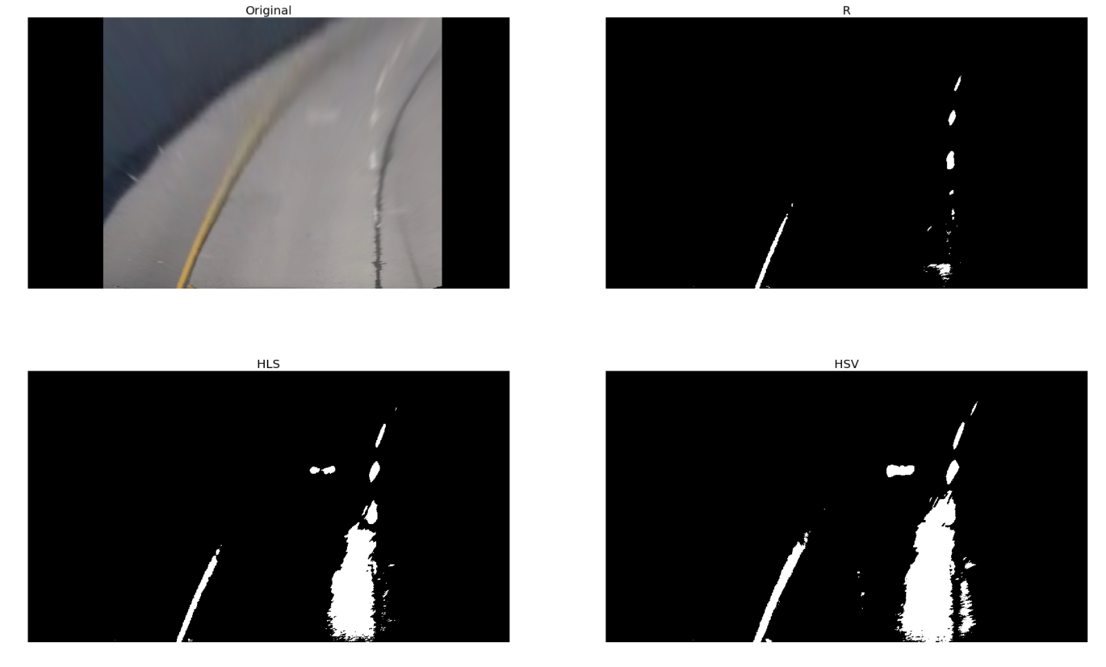
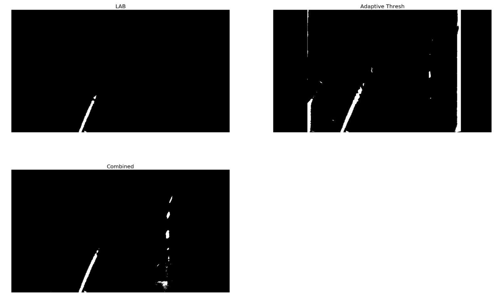
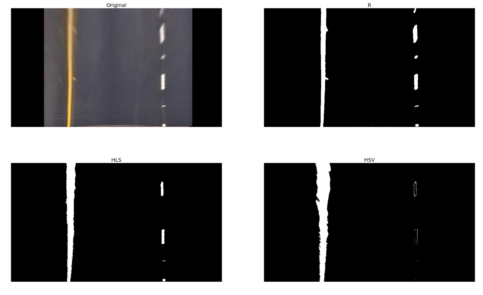
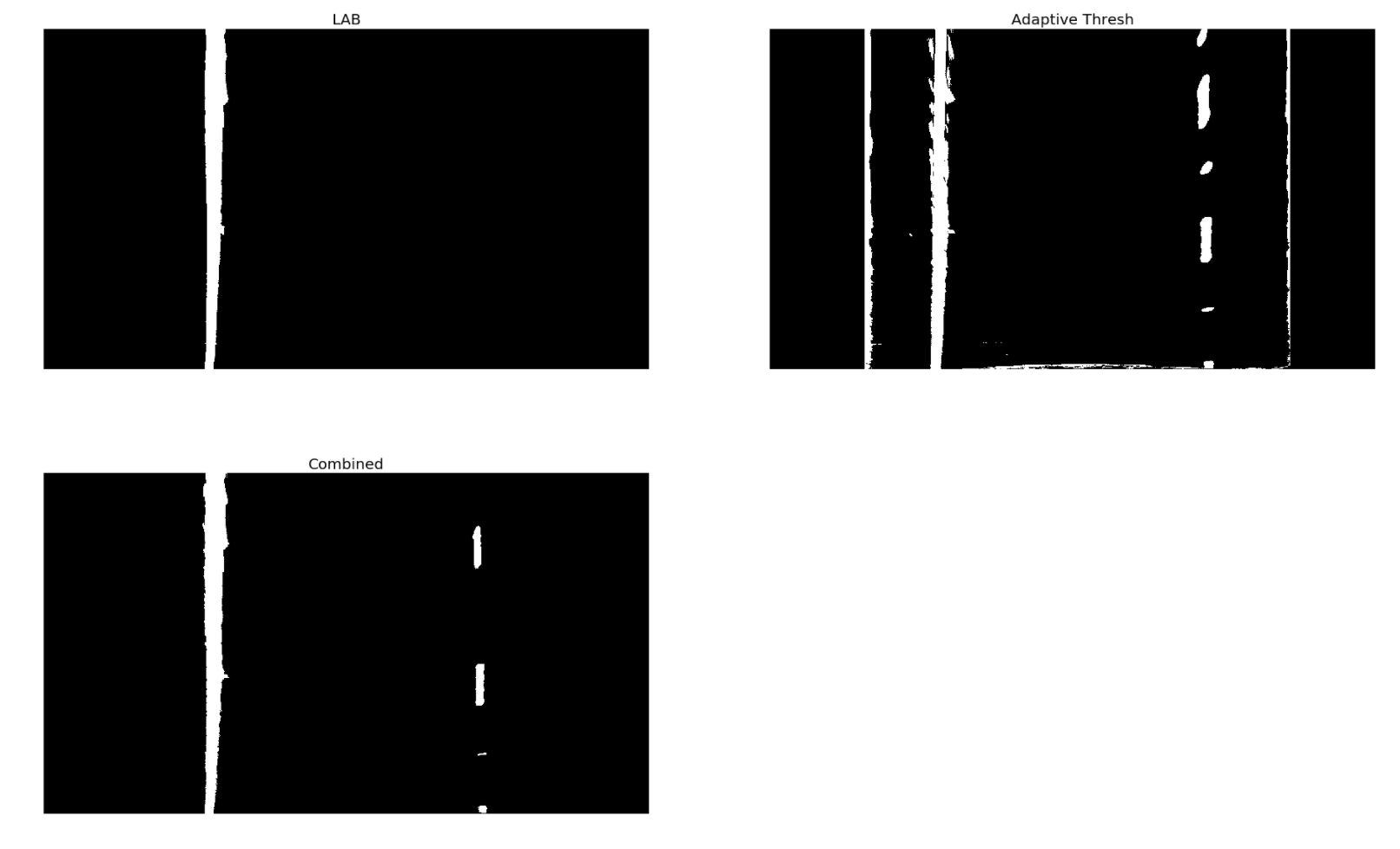
Five masks were used, namely, RGB, HLS, HSV, LAB and a custom adaptive mask
-
Each of these masks were composed through a Logical OR of two sub-masks created to detect the two lane line colors of yellow and white. Moreover, the threshold values associated with each sub-mask was adaptive to the mean of image / search window (further details on the search window has been provided in the sub-sections below)
Logically, this can explained as:
Mask = Sub-mask (white) | Sub-mask (yellow) -
The custom adaptive mask used in the ensemble leveraged the OpenCV
cv2.adaptiveThresholdAPI with a Gaussian kernel for computing the threshold value. The construction process for the mask was similar to that detailed above with one important mention to the constructuion of the submasks:- White submask was created through a Logical AND of RGB R-channel and HSV V-channel, and,
- Yellow submask was created through a Logical AND of LAB B-channel and HLS S-channel
The image below showcases the masking operation and the resulting thresholded binary image from the ensemble for two test images.
An important mention to the reader is that the use of the ensemble gave a ~15% improvement in pixel detection over using just an individual color mask.
We now have a warped, thresholded binary image where the pixels are either 0 or 1; 0 (black color) constitutes the unfiltered pixels and 1 (white color) represents the filtered pixels. The next step involves mapping out the lane lines and determining explicitly which pixels are part of the lines and which belong to the left line and which belong to the right line.
The first technique employed to do so is: Peaks in Histogram & Sliding Windows
-
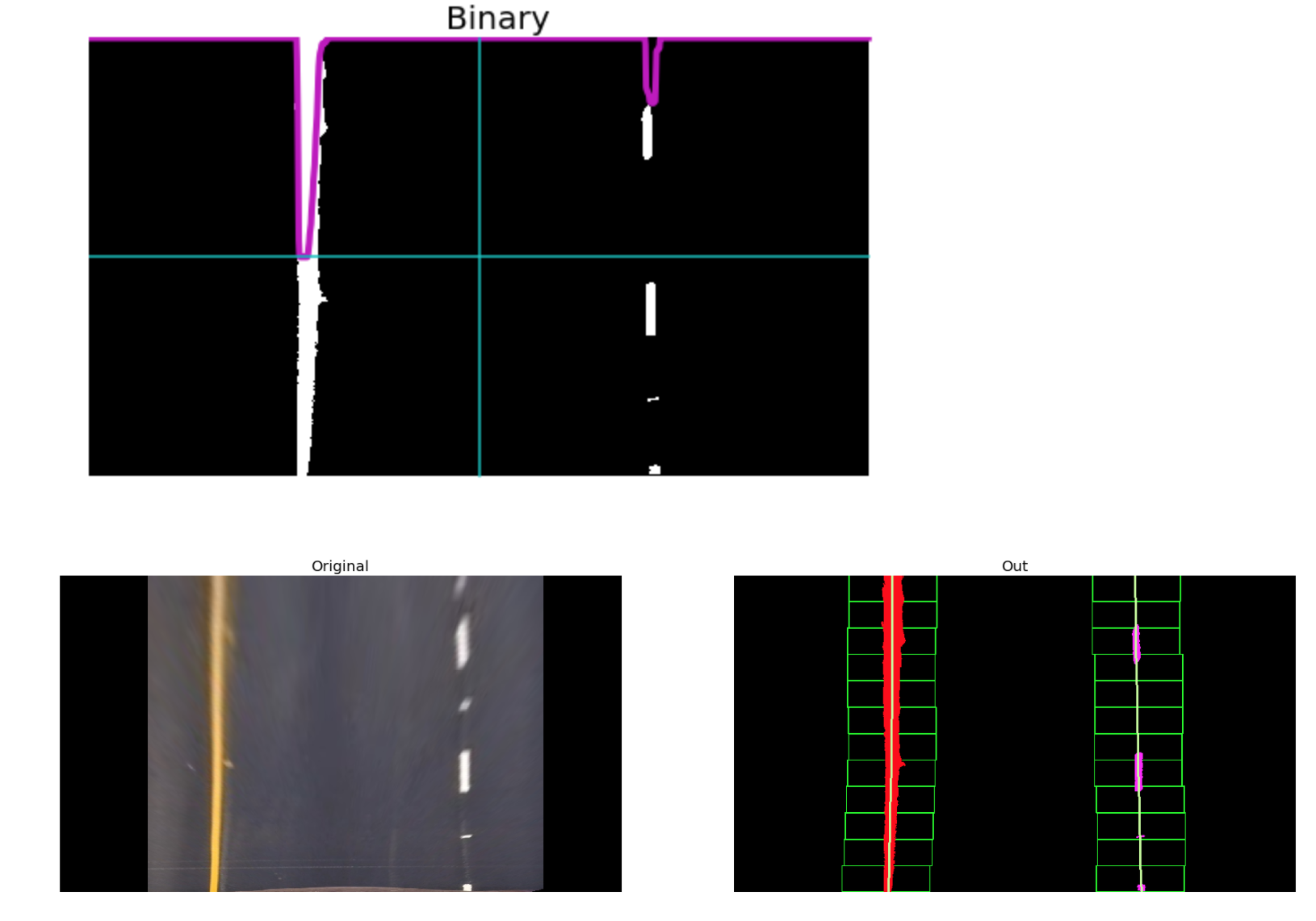
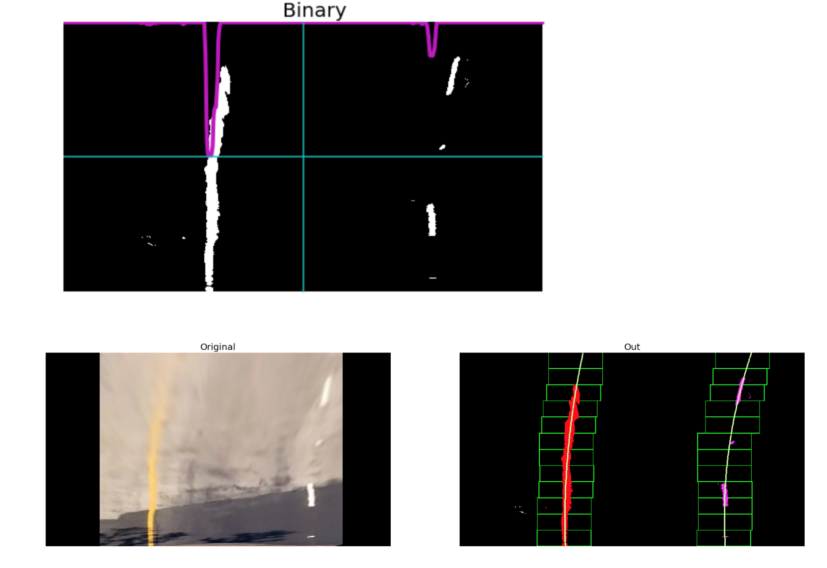
We first take a histogram along all the columns in the lower half of the image. This involves adding up the pixel values along each column in the image. The two most prominent peaks in this histogram will be good indicators of the x-position of the base of the lane lines. These are used as starting points for our search.
-
From these starting points, we use a sliding window, placed around the line centers, to find and follow the lines up to the top of the frame.
The parameters used for the sliding window search are:
   nb_windows = 12 # number of sliding windows
   margin = 100 # width of the windows +/- margin
   minpix = 50 # min number of pixels needed to recenter the window
   min_lane_pts = 10  # min number of 'hot' pixels needed to fit a 2nd order polynomial as a lane line
The 'hot' pixels that we have found are then fit to a second order polynomial. The reader should note that we are fitting for y as opposed to x since the lines in the warped image are near vertical and may have the same x value for more than one y value. Once we have computed the 2nd order polynomial coefficients, the line data is obtained for y ranging from (0, 720 i.e. image height) by using the mathematical formula:
x = f(y) = Ay^2 + By + C
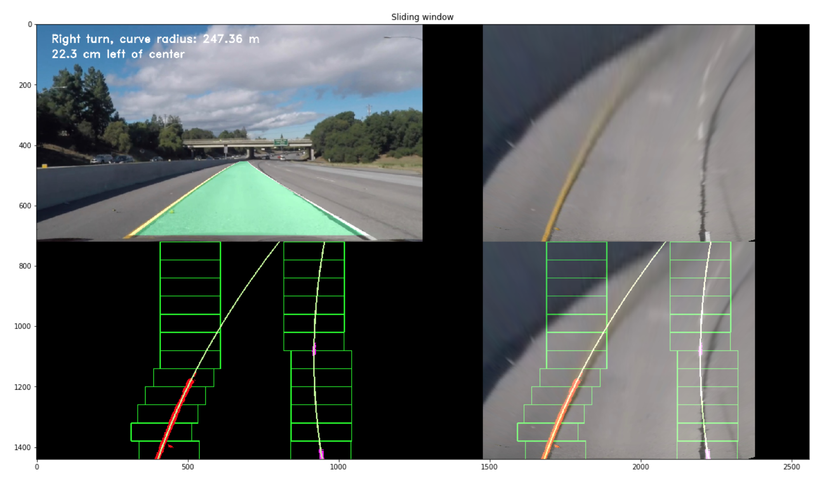
A visualisation of this process can be seen below.
Here, the red and pink color represents the 'hot' pixels for the left and right lane lines respectively. Furthermore, the line in green is the polyfit for the corresponding 'hot' pixels.
Once we have successfully detected the two lane lines, for subsequent frames in a video, we search in a margin around the previous line position instead of performing a blind search.
Although the Peaks in Histogram and Sliding Windows technique does a reasonable job in detecting the lane line, it often fails when subject to non-uniform lighting conditions and discolouration. To combat this, a method that could perform adaptive thresholding over a smaller receptive field/window of the image was needed. The reasoning behind this approach was that performing adaptive thresholding over a smaller kernel would more effectively filter out our 'hot' pixels in varied conditions as opposed to trying to optimise a threshold value for the entire image.
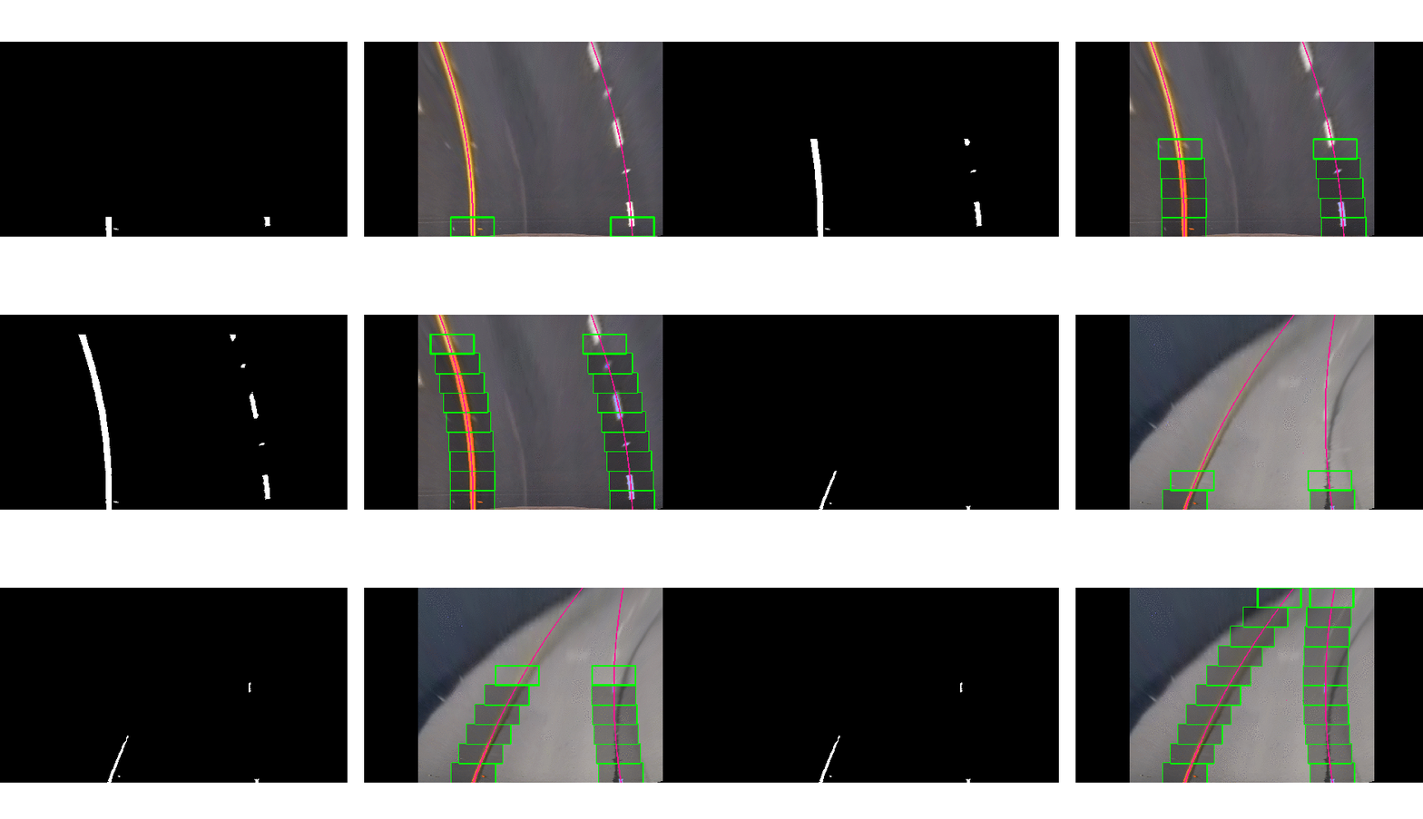
Hence, a custom Adaptive Search technique was implemented to operate once a frame was successfully analysed and a pair of lane lines were polyfit through the Sliding Windows technique. This method:
- Follows along the trajectory of the previous polyfit lines and splits the image into a number of smaller windows.
- These windows are then iteratively passed into the
get_binary_imagefunction (defined in Step 4 of the pipeline) and their threshold values are computed as the mean of the pixel intensity values across the window - Following this iterative thresholding process, the returned binary windows are stacked together to get a single large binary image with dimensions same as that of the input image
An important pre-requisite for this method is that: the polynomial coefficients from the previous frame must be known. Therefore, after each successful detection the correpsonding polynomial coefficient are stored into a global cache, the size for which is defined by the user. Moreover, this cache is also used to reduce the jitter and smooth the poly-curve from one frame to the next.
The parameters used in this method are:
   nb_windows = 10 # Number of windows over which to perform the localised color thresholding
   bin_margin = 80 # Width of the windows +/- margin for localised thresholding
   margin = 60 # Width around previous line positions +/- margin around which to search for the new lines
   smoothing_window = 5 # Number of frames over which to compute the Moving Average
   min_lane_pts = 10  # min number of 'hot' pixels needed to fit a 2nd order polynomial as a lane line
A visualisation of this process has been showcased below.
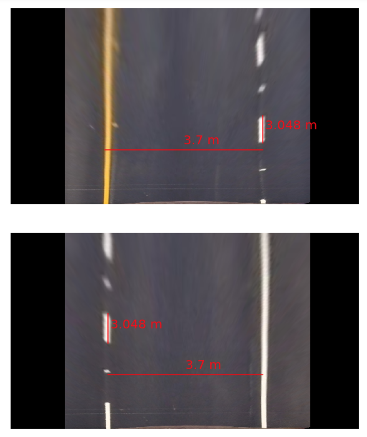
To report the lane line curvature in metres we first need to convert from pixel space to real world space. For this, we measure the width of a section of lane that we're projecting in our warped image and the length of a dashed line. Once measured, we compare our results with the U.S. regulations (as highlighted here) that require a minimum lane width of 12 feet or 3.7 meters, and the dashed lane lines length of 3.048 meters.
The values for metres/pixel along the x/y direction are therefore:
Average meter/px along x-axis: 0.0065
Average meter/px along y-axis: 0.0291
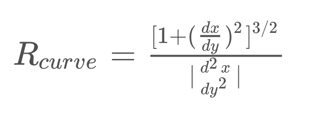
Following this conversion, we can now compute the radius of curvature (see tutorial here) at any point x on the lane line represented by the function x = f(y) as follows:
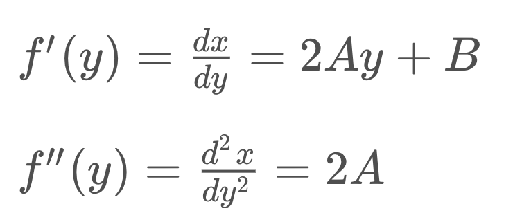
In the case of the second order polynomial above, the first and second derivatives are:
So, our equation for radius of curvature becomes:
Note: since the y-values for an image increases from top to bottom, we compute the lane line curvature at y = img.shape[0], which is the point closest to the vehicle.
A visualisation for this step can be seen below.
An image processing pipeline is therefore setup that runs the steps detailed above in sequence to process a video frame by frame. The results of the pipeline on two test videos can be visualised in the project_video_output.mp4 and challenge_video_output.mp4
An example of a processed frame has been presented to the reader below.
This was a very tedious project which involved the tuning of several parameters by hand. With the traditional Computer Vision approach I was able to develop a strong intuition for what worked and why. I also learnt that the solutions developed through such approaches aren't very optimised and can be sensistive to the chosen parameters. As a result, I developed a strong appreciation for Deep Learning based approaches to Computer Vision. Although, they can appear as a black box at times Deep learning approaches avoid the need for fine-tuning these parameters, and are inherently more robust.
The challenges I encountered were almost exclusively due to non-uniform lighting conditions, shadows, discoloration and uneven road surfaces. Although, it wasn't difficult to select the thresholding parameters to successfully filter the lane pixels it was very time consuming. Furthermore, the two biggest problem with my pipeline that become evident in the harder challenge video are:
-
Its inability to handle sharp turns and constantly changing slope of the road. This a direct consequence of the assumption made in Step 2 of the pipeline where the road in front of the vehicle is assumed to be relatively flat and straight(ish). This results in a 'static' perspective transformation matrix meaning that if the assumption doesn't hold true the lane lines will no longer be relatively parallel. As a result, it becomes a lot harder to assess the validity of the detected lane lines, because even if the lane lines in the warped image are not nearly parallel, they might still be valid lane lines.
-
Poor lane lines detection in areas of glare/ severe shadows / combination of both. This results from the failure of the thresholding function to successfully filter out the lane pixels in these extreme lighting conditions
In the coming weeks, I aim to tackle these problems and improve the performance of the model on the harder challenge video.
- The major challenge we faced was in selection of the color space. It was very essential to detect the lane lines properly.
- The second, most difficult challenge we faced, was choosing the approach for further processing. Whether to go with Hough transform, or to go with histogram method and polynomial fitting. After experimenting with both the approaches, we concluded that histogram of lane pixels approach.
- Some other challenges we faced were in the sliding window approach, and in the polynomial fitting. The sliding window kept coming back to the center of the image because the histogram couldn’t have the right peak in it. This was corrected by re-choosing the four points taken to obtain the birds eye view.

