SQL-INTERVIEW-QUESTIONS

Keys in DBMS

KEYS in DBMS is an attribute or set of attributes which helps you to identify a row(tuple) in a relation(table)

Primary key

Primary key is a set of one or more columns of a table that uniquely identify a record in a database table. It can not accept null, duplicate values.
Candidate key

A Candidate Key is a set of one or more columns that can identify a record uniquely in a table. There can be multiple Candidate Keys in one table. Only one Candidate Key can be Primary Key
Unique key

A unique key is a set of one or more columns of a table that uniquely identify a record in a database table. It is like Primary key but it can accept only one null value and it cannot have duplicate values
Alternate key

An Alternate key is a key that can be work as a primary key. Basically, it is a candidate key that currently is not a primary key.

Example: In a table, RollNo and EnrollNo become Alternate Keys when we define ID as Primary Key.
Super key

Super key is a set of one or more than one keys that can be used to identify a record uniquely in a table. Example: Primary key, Unique key, Alternate key are a subset of Super Keys.
Composite/Compound Key

Composite Key is a combination of more than one fields/columns of a table. It can be a Candidate key, Primary key.
Foreign Key

Foreign Key is a field in a database table that is Primary key in another table

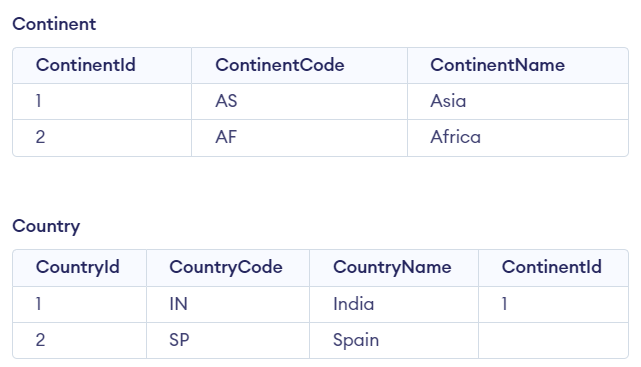
SQL Joins

SQL Join statement is used to combine data or rows from two or more tables based on a common field between them.
1. INNER JOIN
  
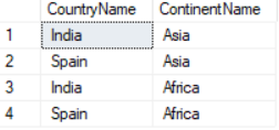
  The INNER JOIN keyword selects all rows from both the tables as long as the condition satisfies
```
SELECT cr.CountryName, ct.ContinentName
FROM Country cr
INNER JOIN  Continent ct ON ct.ContinentId = cr.ContinentId;
```
  Result:
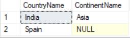
2. LEFT JOIN
  
  The LEFT JOIN returns all the rows of the table on the left side of the join and matching rows for the table on the right side of join.
```
SELECT cr.CountryName, ct.ContinentName
FROM Country cr
LEFT JOIN  Continent ct ON ct.ContinentId = cr.ContinentId;
```
  Result:
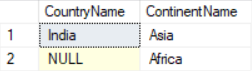
3. RIGHT JOIN
  
  The RIGHT JOIN returns all the rows of the table on the right side of the join and matching rows for the table on the left side of join.
```
SELECT cr.CountryName, ct.ContinentName
FROM Country cr
RIGHT JOIN  Continent ct ON ct.ContinentId = cr.ContinentId;
```
  Result:
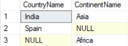
4. FULL JOIN
  
  The FULL JOIN returns all the rows from both the tables. The rows for which there is no matching, the result-set will contain NULL
```
SELECT cr.CountryName, ct.ContinentName
FROM Country cr
FULL JOIN  Continent ct ON ct.ContinentId = cr.ContinentId;
```
  Result:
5. CROSS JOIN
  
  CROSS JOIN joins all the records from left table with all the records from right table. It is not based on matching any column. ON is not required. Result row count is number of records in left table multiplied by number of records in right table (Cartesian product)
```
SELECT cr.CountryName, ct.ContinentName
FROM Country cr
CROSS JOIN  Continent ct ;
```
  Result:
6. NATURAL JOIN
  
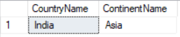
  NATURAL JOIN is similar to INNER join but we do not need to use the ON clause during the join. SQL joins two tables based on the common column name in these two tables.
  Both tables must have columns with same name and same data type. (eg: Here ContinentId)
  
  It is not allowed in MS SQL Server
```
SELECT cr.CountryName, ct.ContinentName
FROM Country cr
NATURAL JOIN  Continent ct
```
  Result:
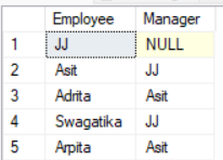
7. SELF JOIN
  
  SELF JOIN is when we join a table to itself. We just use the normal INNER/LEFT join to do a self join with the table having different alias name.
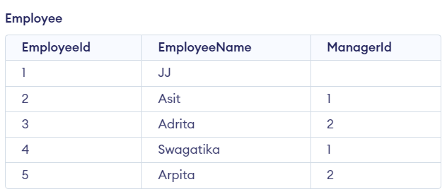
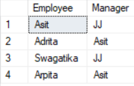
```
  SELECT
  	emp.EmployeeName as Employee,
  	mng.EmployeeName as Manager
  FROM Employee emp 
  JOIN Employee mng ON emp.ManagerId = mng.EmployeeId
```
  Result:
```
  SELECT
  	emp.EmployeeName as Employee,
  	mng.EmployeeName as Manager
  FROM Employee emp 
  LEFT JOIN Employee mng ON emp.ManagerId = mng.EmployeeId
```
  Result:
Difference between DROP and DELETE/TRUNCATE

DROP is used to remove the entire table screma from the DB whereas DELETE/TRUNCATE is used to only remove records

Difference between DELETE and TRUNCATE

Delete can be used to remove either few or all the records from a table	Truncate will always remove all the records from the table. Truncate cannot have WHERE condition
Delete is a DML statement hence we will need to commit the transaction in order to save the changes to database	Truncate is a DDL statement hence no commit is required
Speed is slow because it maintains transaction logs for each deleted record.	It's execution is fast because it deletes entire data at a time without maintaining transaction logs.
Doesn't reset the table identity because it only deletes the data	It always resets the table identity.
Requires DELETE permission to use this command.	Requires ALTER permission to use this command.

Difference between UNION and UNION ALL

UNION and UNION ALL are SQL operators used to concatenate 2 or more result sets. This allows us to write multiple SELECT statements, retrieve the desired results, then combine them together into a final, unified set.

The main difference between UNION and UNION ALL is that:
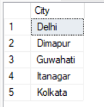
- UNION: only keeps unique records
- UNION ALL: keeps all records, including duplicates
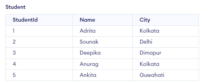
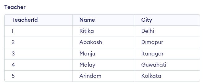
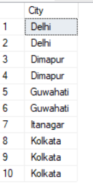
```
SELECT City FROM Student  
UNION  
SELECT City FROM Teacher  
ORDER BY City;  
	
```
Result:
```
SELECT City FROM Student  
UNION ALL
SELECT City FROM Teacher  
ORDER BY City;  
	
```
Result:
Window functions in SQL

Window functions applies aggregate and ranking functions over a particular window (set of rows).

AGGREGATE FUNCTIONS
- AVERAGE
NULL is ignored. In both the cased the items are divided by 3 and threfore same result 2.
```
CREATE TABLE #ITEMS (Num INT)

INSERT INTO #ITEMS VALUES (1), (2) , (3)  

SELECT
	AVG(Num) 
FROM #ITEMS

TRUNCATE table #ITEMS

INSERT INTO #ITEMS VALUES (1), (2) ,(null), (3)  

SELECT
	AVG(Num) 
FROM #ITEMS
```
- SUM
- MIN
- MAX
- COUNT
- GROUP BY
The GROUP BY statement groups rows that have the same values into summary rows. It is mostly used when the user request needs "by" or "for each"
```
SELECT 
	e.DepartmentId,
	MAX(d.DepartmentName) as DepartmentName,
	Count(*) AS EmpCount
FROM Employee e
JOIN Department d on e.DepartmentId = d.DepartmentId
GROUP BY e.DepartmentId
```
Example:
- Total sales by product category
- Average sale for each customer
ROLL UP

Ranking Window Functions

Window functions applies aggregate and ranking functions over a particular window (set of rows). OVER clause is used with window functions to define that window. OVER clause does two things :
- Partitions rows into form set of rows. (PARTITION BY clause is used)
- Orders rows within those partitions into a particular order. (ORDER BY clause is used)
Basic Syntax :
```
SELECT coulmn_name1, 
 window_function(cloumn_name2),
 OVER([PARTITION BY column_name1] [ORDER BY column_name3]) AS new_column
FROM table_name;


window_function= any aggregate or ranking function    
column_name1= column to be selected
coulmn_name2= column on which window function is to be applied
column_name3= column on whose basis partition of rows is to be done
new_column= Name of new column
table_name= Name of table	
```
1. Ranking :
  
  Ranking functions are, RANK(), DENSE_RANK(), ROW_NUMBER()
  
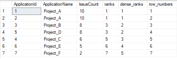
  RANK() function will assign a rank to each row within each partitioned result set. If multiple rows have the same value then each of these rows will share the same rank. However the rank of the following (next) rows will get skipped. Meaning for each duplicate row, one rank value gets skipped. Rank is assigned such that rank 1 given to the first row and rows having same value are assigned same rank.
  
  DENSE_RANK() assigns rank to each row within partition. Just like rank function first row is assigned rank 1 and rows having same value have same rank. The difference between RANK() and DENSE_RANK() is that in DENSE_RANK(), for the next rank after two same rank, consecutive integer is used, no rank is skipped.
  
  ROW_NUMBER() assigns consecutive integers to all the rows within partition. Within a partition, no two rows can have same row number.
  
  ApplicationIssue
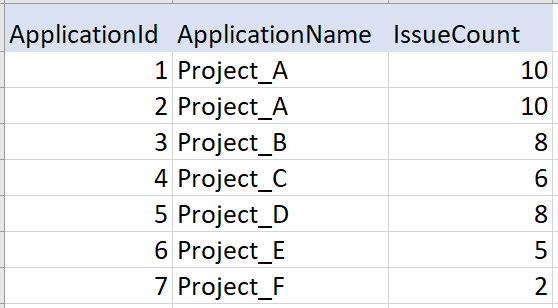
```
SELECT *,
  RANK() OVER(ORDER BY IssueCount DESC) AS ranks,
  DENSE_RANK() OVER(ORDER BY IssueCount DESC) AS dense_ranks,
  ROW_NUMBER() OVER(ORDER BY IssueCount DESC) AS row_numbers
FROM ApplicationIssue;
```
  Output:
SubQuery/ WITH

Subquery means query within a query. It should return single scalar value.
- Breakdown complex logic
- Use in places where joins aren' tallowed (Joins are faster)
- SQL server frequently rewrites subqueries as join. We can use subquery for better readability
We can put subquery in:

SELECT line :
```
SELECT
	ProductName,
	Price,
	Price - (SELECT AVG(Price) FROM Product) as DifferenceFromAverage
FROM Product	
```
WHERE line :
```
SELECT
	ProductName,
	Price
FROM Product
WHERE
	ProductId IN (SELECT ProductId FROM DaiyProductOffer)
```
FROM line :

Predicates Used with Subqueries
- IN
- EXISTS (EXISTS is faster than IN)
  
  SELECT ProductName, Price FROM Product AS P WHERE EXISTS (SELECT ProductId FROM DaiyProductOffer offer WHERE offer.ProductId = p.ProductId )
- ALL
- ANY
- SOME
Common table expression (CTE)

A CTE is a temporary result set, that can be referenced within a SELECT, INSERT, UPDATE, or DELETE statement, that immediately follows the CTE.
- Breakdown complex queries
- Avoid subqueries
- Simplify certain syntax
Syntax
```
WITH cte_name (Column1, Column2, ..)
AS
( CTE_query )
```
Requirement:

We have Employee and Department tables:

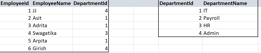
Get Employee count in each department.
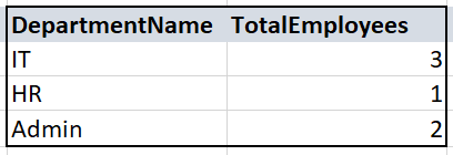
```
WITH EmployeeCount(DepartmentId, TotalEmployees)
as
(
	SELECT 
		DepartmentId, 
		COUNT(*) as TotalEmployees
	FROM Employee
	GROUP BY DepartmentId
)

SELECT
	d.DepartmentName, 
	cnt.TotalEmployees
FROM Department d
JOIN EmployeeCount cnt
on d.DepartmentId = cnt.DepartmentId
```
Here the CTE output is following, the output is joines with Department.

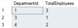
The overall OUTPUT is:
Merge

PIVOT and UNPIVOT

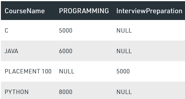
PIVOT operator converts the rows data of the table into the column data.

We have a table Course

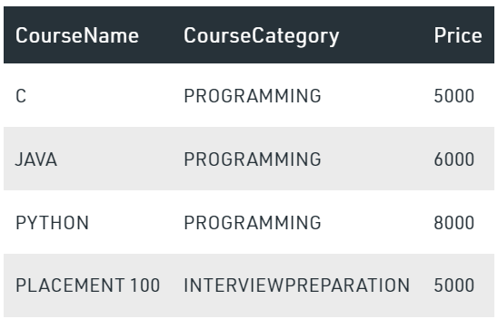
SELECT CourseName, PROGRAMMING, INTERVIEWPREPARATION
FROM Course 
PIVOT 
( 
	SUM(Price) FOR CourseCategory IN (PROGRAMMING, INTERVIEWPREPARATION ) 
) AS PivotTable

Output:

UNPIVOT transforms the column based data into rows

Performance Tuning
Index

SQL Indexes are used in relational databases to quickly retrieve data. They are similar to indexes at the end of the books whose purpose is to find a topic quickly. The existence of the right indexes, can drastically improve the performance of the query.
- Data is internally stored in a SQL Server database in “pages” where the size of each page is 8KB.
- A continuous 8 pages is called an “Extent”.
- When we create the table then one extent will be allocated for two tables and when that extent is is filled with the data then another extent will be allocated and this extent may or may not be continuous to the first extent.
- If there is no index, then the query engine, checks every row in the table from the beginning to the end. This is called as Table Scan. Table scan is bad for performance
Index Example:

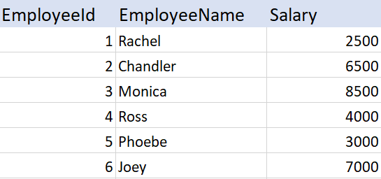
At the moment, the table, does not have an index on SALARY column. Considering the following query:
```
Select * from EmployeeSalary where Salary > 3000 and Salary < 7000	
```
The query engine has to check each and every row in the table, resulting in a table scan, which can adversely affect the performance, especially if the table is large. To create an index on Salary column :
```
CREATE Index IX_EmployeeSalary_Salary 
ON EmployeeSalary (SALARY ASC)	
```
The index stores salary of each employee, in the ascending order as shown below. The actual index may look slightly different.

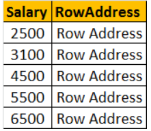
Now, when the SQL server has to execute the same query, it has an index on the salary column to help this query. Salaries between the range of 3000 and 7000 are usually present at the bottom, since the salaries are arranged in an ascending order. SQL server picks up the row addresses from the index and directly fetch the records from the table, rather than scanning each row in the table. This is called as Index Seek.

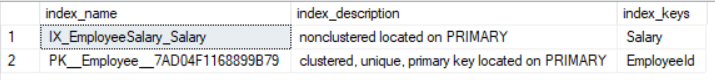
To view all index of a table :
```
sp_Helpindex EmployeeSalary
```
To delete or drop the index:
```
Drop Index EmployeeSalary.IX_EmployeeSalary
```
Output:

Different types of indexes
1. Clustered
2. Nonclustered
3. Unique
4. Filtered
5. XML
6. Full Text
7. Spatial
8. Columnstore
9. Index with included columns
10. Index on computed columns
Clustered Index:

A clustered index determines the physical order of data in a table based on which data will be arranged. A table can have only one clustered index
Primary key, constraint create clustered indexes automatically if no clustered index already exists on the table
```
Insert into EmployeeSalary Values(3,'John',4500)
Insert into EmployeeSalary Values(1,'Sam',2500)
Insert into EmployeeSalary Values(4,'Sara',5500)
Insert into EmployeeSalary Values(5,'Todd',3100)
Insert into EmployeeSalary Values(2,'Pam',6500)									  
```
Inspite, of inserting the rows in a random order, when we execute the select query we can see that all the rows in the table are arranged in an ascending order based on the Id column

Deleting Clustered Index:
```
Drop index tblEmployee.PK__tblEmplo__3214EC070A9D95DB
```
When you execute this query, you get an error message stating 'An explicit DROP INDEX is not allowed on index 'tblEmployee.PK__tblEmplo__3214EC070A9D95DB'. It is being used for PRIMARY KEY constraint enforcement.' To successfully delete the clustered index, right click on the index in the Object explorer window and select DELETE.

Composite clustered Index

A table can have only one clustered index. However, the index can contain multiple columns (a composite index)
```
Create Clustered Index IX_tblEmployee_Gender_Salary
ON tblEmployee(Gender DESC, Salary ASC)
```
select query against this table you should see the data physically arranged, FIRST by Gender in descending order and then by Salary in ascending order.

Non Clustered Index:

In a nonclustered index, the data is stored in one place, the index in another place. The index will have pointers to the storage location of the data. Since, the nonclustered index is stored separately from the actual data, a table can have more than one non clustered index,
Execution Plan

Execution plan in SQL Server Management Studio is a graphical representation of the various steps that are involved in fetching results from the database tables. Once a query is executed, the query processing engine quickly generates multiple execution plans and selects the one which returns the results with the best performance.

There are two types of execution plans –

Estimated Execution Plan

It is just a guess by the query processor about how the specific steps that are to be involved while returning the results. It is generated before the query has been executed.

Actual Execution Plan

It is generated after the query has been executed. It shows the actual operations and steps involved while executing the query. This may or may not differ from the Estimated Execution Plan

Common SQL Queries

Find and Delete Duplicate records from a table

CustomerId	FirstName	LastName	Email
1	Adrita	Sharma	adritasharma@gmail.com
2	Sounak	Chakraborty	chakraborty.sounak@gmail.com
3	Deepika	Das	das.deepika31@gmail.com
4	Ankita	Sarkar	ankitasarkar1994@gmail.com
5	Anurag	Shyam	anurag1994@gmail.com
6	Sounak	Chakraborty	chakraborty.sounak@gmail.com
7	Deepika	Das	das.deepika31@gmail.com

A) USING SELF JOIN

Finding duplicate rows:

SELECT *
FROM
	CUSTOMER C1
	JOIN CUSTOMER C2 ON C1.Email = C2.Email
WHERE 
	C2.CustomerId > C1.CustomerId

Deleting duplicate rows:

DELETE C2
FROM
	CUSTOMER C1
	JOIN CUSTOMER C2 ON C1.Email = C2.Email
WHERE 
	C2.CustomerId > C1.CustomerId

B) USING GROUP BY

Finding duplicate rows:

SELECT 
	Email, Count(*) as Cnt
FROM CUSTOMER
GROUP BY Email
HAVING Count(*) > 1

Deleting duplicate rows:

DELETE FROM CUSTOMER
WHERE 
	CustomerId IN (
		SELECT 
			Max(CustomerId)
		FROM CUSTOMER
		GROUP BY Email
		HAVING Count(*) > 1
	)

C) USING ROW_NUMBER() & PARTITION BY -- Used when there is no Primary Key Id

Finding duplicate rows:

SELECT 
    Email,
    ROW_NUMBER() OVER (
        PARTITION BY 
           Email
        ORDER BY 
           Email
    ) row_num
 FROM 
    CUSTOMER

O/P

Email	row_num
adritasharma@gmail.com	1
ankitasarkar1994@gmail.com	1
anurag1994@gmail.com	1
chakraborty.sounak@gmail.com	1
chakraborty.sounak@gmail.com	2
das.deepika31@gmail.com	1
das.deepika31@gmail.com	2

Deleting duplicate rows:

WITH cte AS (
	SELECT 
		Email,
		ROW_NUMBER() OVER (
			PARTITION BY 
			Email
			ORDER BY 
			Email
		) row_num
	FROM 
		CUSTOMER
)
DELETE FROM cte WHERE row_num > 1;

Second Highest Salary

EmployeeId	Salary
1	2500
5	3000
4	4000
2	6500
6	7000
3	8500

A) USING INNER QUERY

SELECT MAX(Salary)
FROM EmployeeSalary
WHERE Salary < (SELECT MAX(Salary)	FROM EmployeeSalary)

B) Finding Lowest of TOP 2

SELECT TOP 2 Salary FROM EmployeeSalary ORDER BY Salary DESC

o/p

Salary
8500
7000

WITH cte AS (
	SELECT TOP 2 Salary FROM EmployeeSalary ORDER BY Salary DESC
)

SELECT Min(Salary) FROM cte;

C) USING DENSE_RANK()

SELECT 
		Salary,
		DENSE_RANK() OVER (
			ORDER BY Salary Desc
		) as Rnk
FROM EmployeeSalary

o/p

Salary	Rnk
8500	1
7000	2
6500	3
4000	4
3000	5
2500	6

WITH cte AS (
	SELECT 
		Salary,
		DENSE_RANK() OVER (
			ORDER BY Salary Desc
		) as Rnk
	FROM EmployeeSalary
)
SELECT Salary FROM cte WHERE Rnk = 2;

nth Highest Salary

A) USING DENSE_RANK()

WITH cte AS (
	SELECT 
		Salary,
		DENSE_RANK() OVER (
			ORDER BY Salary Desc
		) as Rnk
	FROM EmployeeSalary
)
SELECT Salary FROM cte WHERE Rnk = 4;

B) Finding Lowest of TOP n

CREATE FUNCTION Get_Nth_Highest_Salary(@n int)

RETURNS TABLE 
AS
RETURN 
(
	WITH cte AS (
	SELECT TOP (@n) Salary FROM EmployeeSalary ORDER BY Salary DESC
	)

	SELECT Min(Salary) as Salary FROM cte
)
GO

Excecuting the fuunction :

SELECT * FROM Get_Nth_Highest_Salary(4)

o/p

Salary
4000

QUERY Performance Improvement

EXISTS is faster than IN

adritasharma/SQL-INTERVIEW-QUESTIONS

SQL-INTERVIEW-QUESTIONS

AGGREGATE FUNCTIONS

Ranking Window Functions

Common SQL Queries

Find and Delete Duplicate records from a table

Second Highest Salary

nth Highest Salary

QUERY Performance Improvement