An R package that uses the air2water model to predict Lake Surface Temperature (LST) using air temperature. Version 2.0.0 - January 2017 - compiled September 2020.
To install air2wateR from Github with:
# install.packages("devtools")
devtools::install_github("aemon-j/air2wateR")
library(air2wateR)

sim_folder <- system.file('extdata', package = 'air2wateR')

# Generate parameters
gen_param(sim_folder = sim_folder, mean_depth = 147)

# Run the model
run_air2water(sim_folder = sim_folder, mode = "pso")
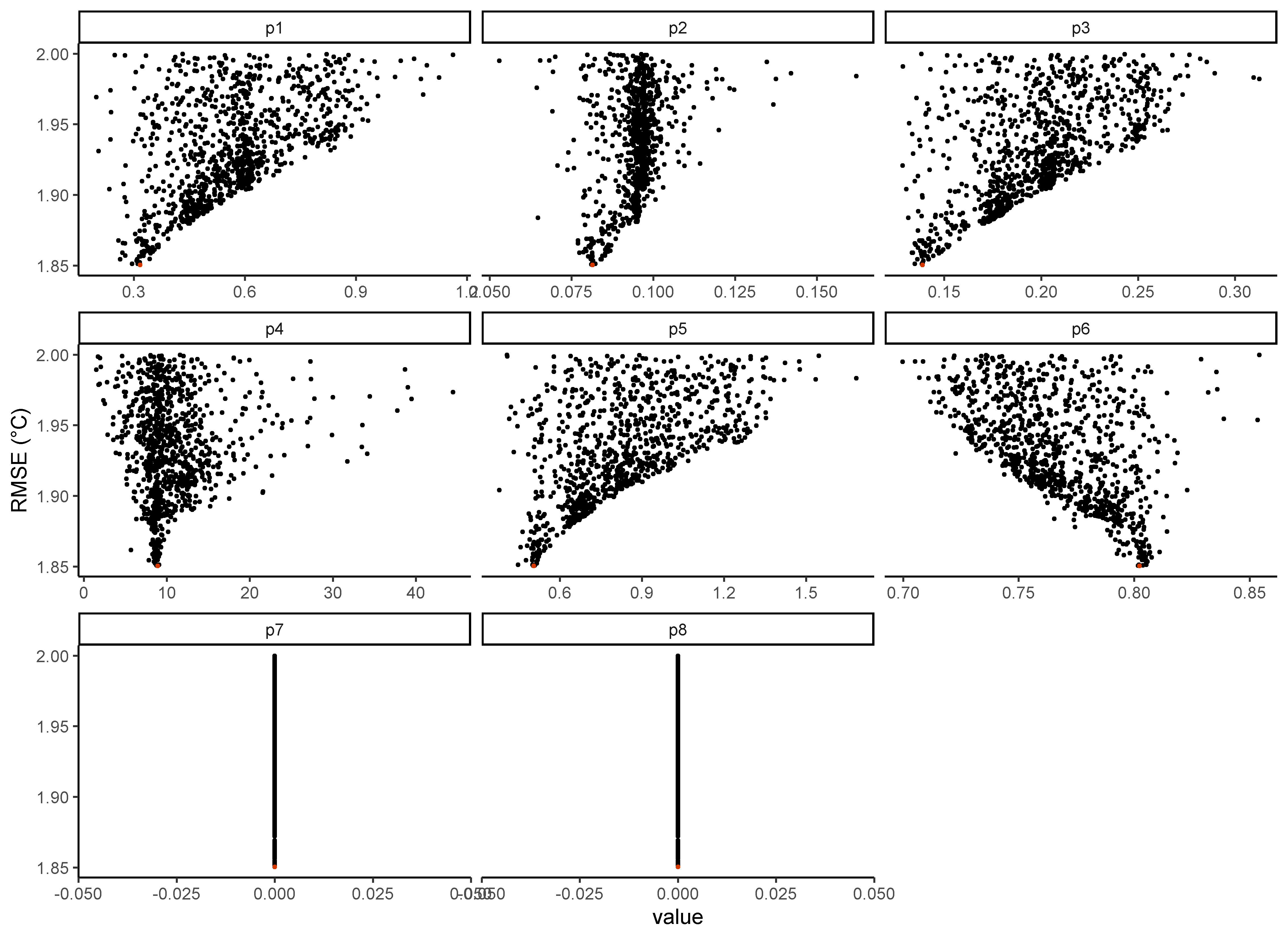
plot_param(sim_folder = sim_folder) +
  ylab('RMSE (\u00B0C)') +
  theme_classic(base_size = 18)
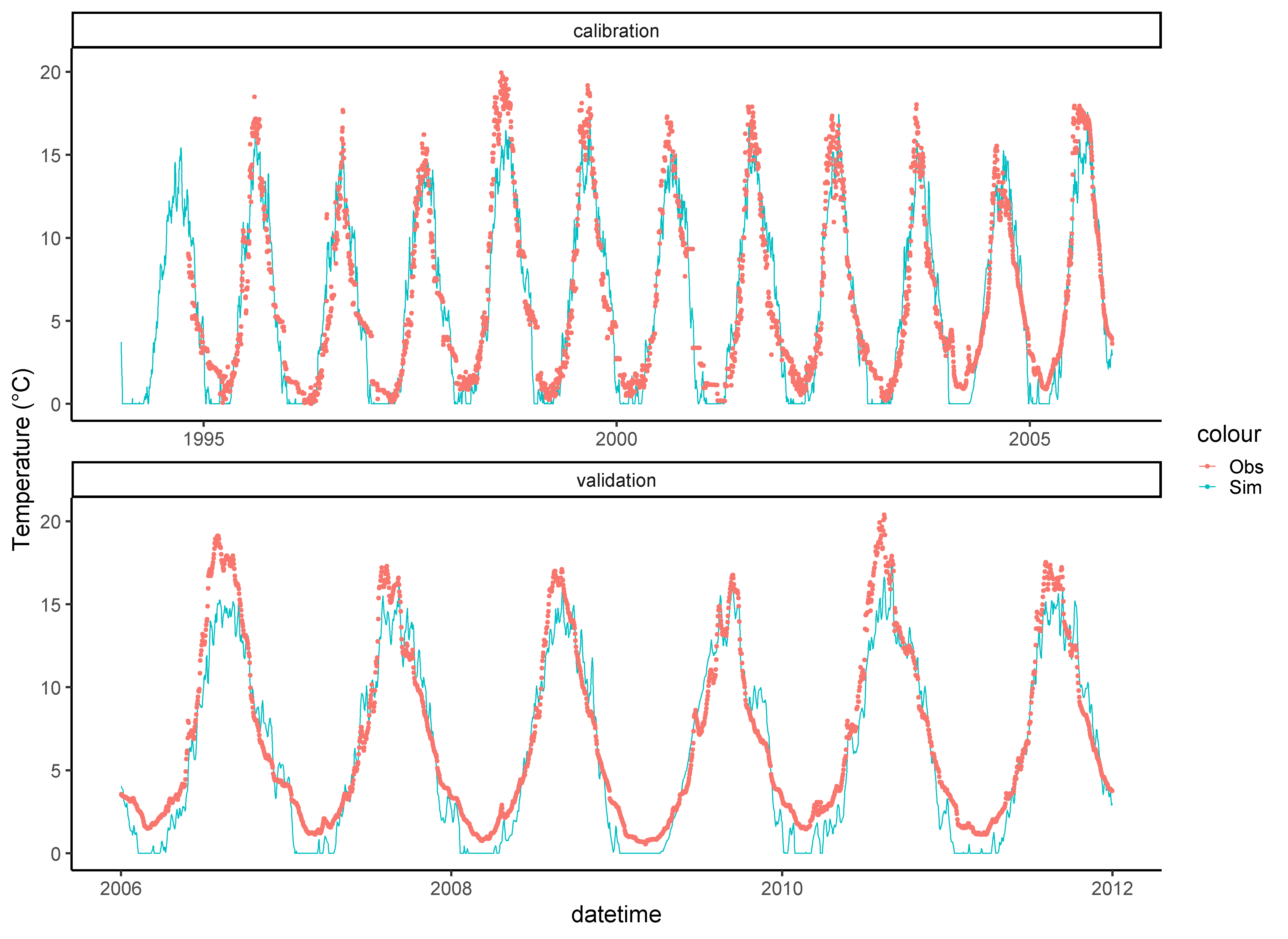
run_air2water(sim_folder = sim_folder, mode = "forward", use_pars = TRUE)
out <- get_outputs(sim_folder = sim_folder)

library(ggplot2)
ggplot(out) +
  geom_line(aes(datetime, LSWT_sim, colour = 'Sim')) +
  geom_point(aes(datetime, LSWT_obs, colour = 'Obs')) +
  facet_wrap(~status, nrow = 2, scales = "free_x") +
  ylab('Temperature (\u00B0C)') +
  theme_classic(base_size = 20)
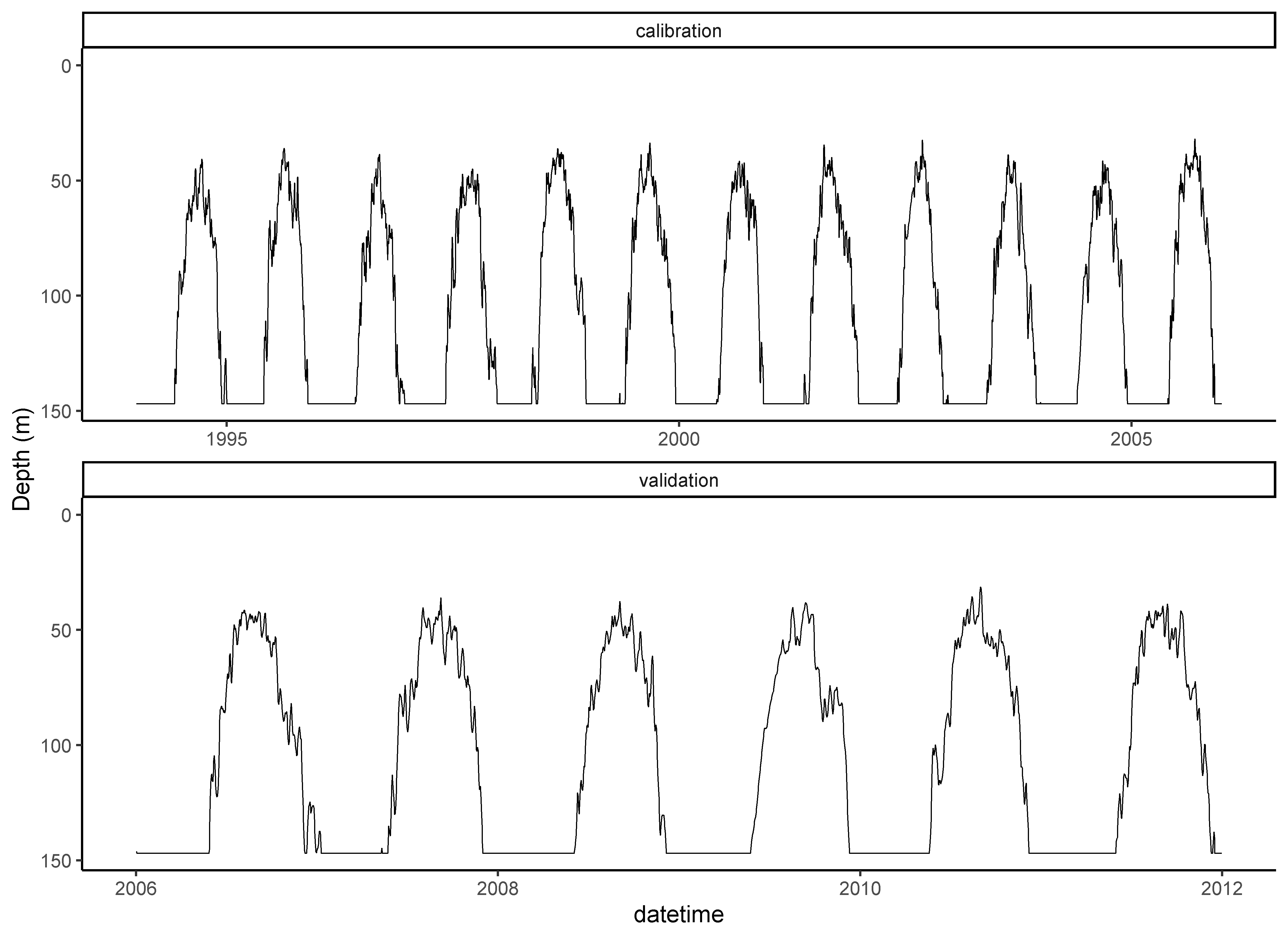
out <- get_outputs(sim_folder = sim_folder)

mean_depth <- 147 # Lake Superior
out$wml <- out$C * mean_depth # estimate well-mixed layer as a function of mean depth

library(ggplot2)
ggplot(out) +
  geom_line(aes(datetime, wml)) +
  facet_wrap(~status, nrow = 2, scales = "free_x") +
  ylab('Depth (m)') +
  scale_y_reverse() +
  coord_cartesian(ylim = c(mean_depth, 0)) +
  theme_classic(base_size = 20)
- Piccolroaz S., M. Toffolon, and B. Majone (2013), A simple lumped model to convert air temperature into surface water temperature in lakes, Hydrol. Earth Syst. Sci., 17, 3323-3338, doi:10.5194/hess-17-3323-2013
- Toffolon M., S. Piccolroaz, B. Majone, A.M. Soja, F. Peeters, M. Schmid and A. Wüest (2014), Prediction of surface water temperature from air temperature in lakes with different morphology, Limnology and Oceanography, 59(6), 2185-2202, doi:10.4319/lo.2014.59.6.2185
- Piccolroaz S., M. Toffolon, and B. Majone (2015), The role of stratification on lakes' thermal response: The case of Lake Superior, Water Resources Research, 51(10), 7878-7894, doi:10.1002/2014WR016555
- Piccolroaz S. (2016), Prediction of lake surface temperature using the air2water model: guidelines, challenges, and future perspectives, Advances in Oceanography and Limnology, 7:36-50, DOI: http://dx.doi.org/10.4081/aiol.2016.5791
- Piccolroaz S., N.C. Healey, J.D. Lenters, S.G. Schladow, S.J. Hook, G.B. Sahoo, and M. Toffolon (2017), On the predictability of lake surface temperature using air temperature in a changing climate: A case study for Lake Tahoe (U.S.A.), Limnology and Oceanography, 63(1), 243-261, doi:10.1002/lno.10626
- Piccolroaz S., R.I. Woolway, C.J. Merchant (2020), Global reconstruction of twentieth century lake surface water temperature reveals different warming trends depending on the climatic zone, Climatic Change, 160, 427–442, doi:10.1007/s10584-020-02663-z
!!!!!!!!!!!!!!! IMPORTANT NOTE: do not change the encoding of input files. They must be ANSI text files. UTF-8 encoded files cannot be read. I suggest using a simple text editor as Notepad++ to modify/create your input files. !!!!!!!!!!!!!!!
#What is new in air2water Version 2.0.0
In this new release, the main improvement concerns:
- Users can now choose among Euler, Runge-Kutta 2nd order, Runge-Kutta 4th order, and Crank-Nicolson numerical schemes to solve the air2water model. The first three schemes are explicit, and in summer, when δ→0, it may happen that a daily time step is too large to adequately integrate the equation of the model, possibly generating numerical instabilities. In order to avoid this situation, an adaptive sub-stepping procedure has been implemented to avoid numerical instabilities when using Runge-Kutta and forward Euler numerical schemes. The last numerical scheme is implicit, 2nd order accurate, and unconditionally stable: a sub-stepping procedure is not required and the daily time step is used for the whole simulation, making it generally faster (but less accurate than Runge-Kutta 4th order) than the previous schemes.
- A new pre-processor is available for evaluating the a-priori range of variation of parameters given the mean depth of a lake.
The model is presented and discussed in Piccolroaz et al. (2013) and in Piccolroaz (2016). The present version of air2water is the one described in Piccolroaz (2016) and in Toffolon et al. (2014), which coincides with the original version (Piccolroaz et al., 2013), except for some differences in the notation of model parameters. The mathematical model is the same.
Pre-compiled executable files are available for Linux (air2water_v2.0.out) and Windows (air2water_v2.0.exe) systems.
The code is provided with an example test case. The study site is Lake Superior and the data have been downloaded from (downloaded data have been pre-processed):
- National Oceanic and Atmospheric Administration’s (NOAA) National Data Buoy Center (NDBC, webpage: http://www.ndbc.noaa.gov/) --> daily air temperature (STDM4 – Stannard Rock station);
- National Oceanic and Atmospheric Administration’s (NOAA) Great Lakes Environmental Research Laboratory (GLERL, webpage: http://www.glerl.noaa.gov/) --> daily lake surface temperature (satellite-derived LST averaged over the whole lake).
IMPORTANT NOTE: do not change the encoding of input files. They must be ANSI text files. UTF-8 encoded files cannot be read. I suggest using a simple text editor as Notepad++.
1.1 -----> 'input.txt' to be located in the same folder of the executable file. This file contains the input information: ! Input file Superior ! name of the lake stndrck ! name/ID of the air temperature station sat ! name/ID of the water temperature station c ! type of series: c=continuous series, m=mean year 1d ! time resolution: 1d=daily, nw=n weeks (n=1,2,...), 1m=monthly 1 ! model version: 1=a2w 4 par; 2=a2w 6 par, 3=a2w 8 par (IMPORTANT NOTE: VERSION CODES ARE DIFFERENT COMPARED TO THOSE USED IN THE PREVIOUS RELEASE) 0 ! Threshold temperature for ice formation RMS ! objective function: RMS (Root Mean Square Error), NSE (Nash-Sutcliffe Efficiency Index), KGE (Kling-Gupta Efficiency Index) RK4 ! mod_num : numerical method used to solve the model equation EUL (Euler Explicit), RK2 (Runge-Kutta 2), RK4 (Runge-Kutta 4), CRN (Crank-Nicolson) PSO ! run mode: PSO (Particle Swarm Optimization), LATHYP (Latin Hypercube), RANSAM (Random Sampling), or FORWARD 0.60 ! minimum percentage of data: 0...1. E.g., when using 1m time resolution, the monthly average is set to NaN if available data during one month are less than this percentage (60% in this case) 2000 ! n_run: number of iterations -999 ! minimum efficiency index (i.e., RMS, NSE, KGE). All model realization with efficiency index greater than this threshold are saved in file 0_... 1 ! log_flag: 1--> parameters 2 and 3 are searched in a logarithmic space; 0--> parameters 2 and 3 are searched in a linear space 0.9 ! Courant number
1.2 -----> 'PSO.txt' to be located in the same folder of the executable file of air2water. This file contains the parameters of PSO: see e.g.: - Kennedy, J., and R. Eberhart (1995), Particle swarm optimization, in Proceedings of IEEE International Conference on Neural Networks, pp. 1942-1948, doi:10.1109/ICNN.1995.488968. - Robinson, J., and Y. Rahmat-Samii (2004), Particle swarm optimization in electromagnetics, IEEE T. Antenn. Propag., 52, 397-407, doi:10.1109/TAP.2004.823969.
! PSO parameters
2000			! number of particles
2 2	   		! c1, c2: constants known as cognitive and social learning factors (used in the equation of motion of particles)
0.9  0.4    ! inertia max and min (used in the equation of motion of particles)
1.3 -----> A folder named as 'IDwater' (e.g., Superior, see the first line in the file input.txt), located in the same folder of the executable file and containing:
  1.3.1 -----> input files for calibration 'IDair_IDwater_typeofseriesc.txt' (e.g., stndrck_sat_cc.txt) and validation 'IDair_IDwat_typeofseriesv.txt' (e.g., stndrck_sat_cv.txt)
		The two files have 5 columns (year, month, day, air temperature, water temperature):

		2001		1		1		-0.125		1.000
		2001		1		2		 0.158		1.155
		2001		1		3		 1.155		-999
		2001		1		4		 3.458		-999
		2001		1		5		10.125		3.254
		...

		NOTE: 	The series of observed air temperature must be complete. It cannot have gaps or no data.
			The series of observed water temperature can contain no-data (-999).
			The series of data must start on the 1st of January. If data are available after that date, air temperature should be reconstructed and the value -999 assigned to water temperature.
			Both series are always at daily time scale, as the equation of the model is solved with daily time step. The model automatically evaluates weekly, multi-weekly, or monthly averages (of water temperature) when using different time scales for model calibration.

  1.3.2 -----> file 'parameters.txt'
		The file contains the range of variation of each parameter of the model. The range of variation of the parameters can be defined on the basis of physical considerations and is strictly lake dependent, thus its reasonable a priori estimation is crucial to obtain reliable results. The range of parameters can be estimated using the equations presented in the Supplementary Material of Piccolroaz (2016) or, visually, from Figure 3 of the same manuscript. A pre-processing function `gen_param()` to evaluate the a priori physical range of model's parameter (see point 3. Pre-processing).
		The structure of the file 'parameters.txt' is the following:

		-0.017   0.00047   0.00069   2   0.005   0   0     0
		 0.100   0.00850   0.02000   6   0.150   1   150   0.5

		The first line contains the minimum value of each parameters, while the second contains the maximum values. There are 8 columns, as the number of parameters.

  1.3.3 -----> file 'parameters_forward.txt'
		The file contains a set of parameters to be used to run the model in forward mode (required only if the model is run in forward), see 10th line of file input.txt . The structure of the file is as follows:

		 0.000284   0.006668   0.006719   2.888324   0.017322   0.212055 148.709752   0.499891
The model writes the output in a folder called 'output_modelversion' (e.g., output_3) located in the same folder of the input files (e.g., Superior). The folder contains:
2.1 -----> file '0_PSO_.......... .out' Binary file that contains a matrix with 9 columns. Each row contains the set of parameters (columns 1-8) and the associated efficiency index (column 9) of each iteration performed by the optimization algorithm. Only the parameter sets that provide an efficiency larger than the minimum efficiency index defined in the file 'input.txt' are saved. Values are saved in double precision. This file allows: a) drawing the dotty plots of parameters to evaluate whether the a priori range of variations of parameters have been reasonably defined (i.e., not too narrow, not too large), b) evaluating whether the optimization (searching) algorithm converged towards the best solution, c) perform uncertainty analyses (when using LATHYP).
2.2 -----> file '1_PSO_.......... .out' ASCII file that contains the best set of parameters (1st line), the value of the efficiency index during the calibration period (2nd line), and the value of the efficiency index during the validation period (if any, 3nd line)
2.3 -----> file '2_PSO_.......... .out' ASCII file containing the results of the calibration period. Row represent time and columns are: year month day observed air temperature observed water temperature simulated water temperature observed water temperature aggregated at the time scale chosen in file 'input.txt' (e.g., 1m) simulated water temperature aggregated at the time scale chosen in file 'input.txt' (e.g., 1m)
Note that the first year is replicated and is used as warm up year to mitigate the influence of initial conditions.
During the warm up year, year, month and day are equal to -999.
2.4 -----> file '3_PSO_.......... .out' ASCII file with the same structure of file '2_PSO... .out' but referred to the validation period.
2.5 -----> file '4_PSO_.......... .out' Delta (dimensionless thickness of the well-mixed surface layer) during the calibration period. Please refer to Toffolon et al. (2014) and Piccolroaz et al., (2015) to see how to convert delta into the dimensional thickness of the well-mixed surface layer.
2.6 -----> file '5_PSO_.......... .out' Delta (dimensionless thickness of the well-mixed surface layer) during the validation period.
A pre-processing function is used gen_param(). This generates a range of variation of model parameters as a function of the mean depth of the lake (from a mean depth of 1 m to a mean depth of 1000 m.
The output of the pre-processing is:
- the file 'parameters.txt' saved in the simulation folder which contains the estimate of the a priori range of variation of model parameters for the mean depth chosen by the user.
The function get_outputs() extracts the datetime, air temperature (AT), observed lake surface water temperature (LSWT_obs), simulated lake surface water temperature (LSWT_sim), the shape number (C), which can be used to estimate the well mixed layer by multiplying by the mean depth, and a status column indicating whether it was part of the calibration or validation period.
A matlab script is available for post-processing. The script ('post_processing.m') is located in the folder 'post_processing'. The output of the script is saved in the same folder where the output of air2water is located. The figures produced by the post-processing script are:
- dotty plots of parameters;
- comparison between observed air temperature, observed water temperature, and simulated water temperature for the calibration period;
- comparison between observed air temperature, observed water temperature, and simulated water temperature for the validation period.
- Important note The range of parameters should be carefully checked during the post-processing step through the analysis of the dotty plots: the cloud of points should be centred within the searching domain, and in any case the best set of parameters should be sufficiently far from the upper and lower a-priori bounds. Exceptions are represented by parameters p6 and p7, see Piccolroaz et al. (2013), Toffolon et al. (2014), and Piccolroaz (2016).
Trento, 2 September, 2017 Sebastiano Piccolroaz s.piccolroaz@unitn.it
Updated 13 September, 2020 Tadhg Moore tadhgm[at]vt.edu


