Awesome CFD solver written in Go
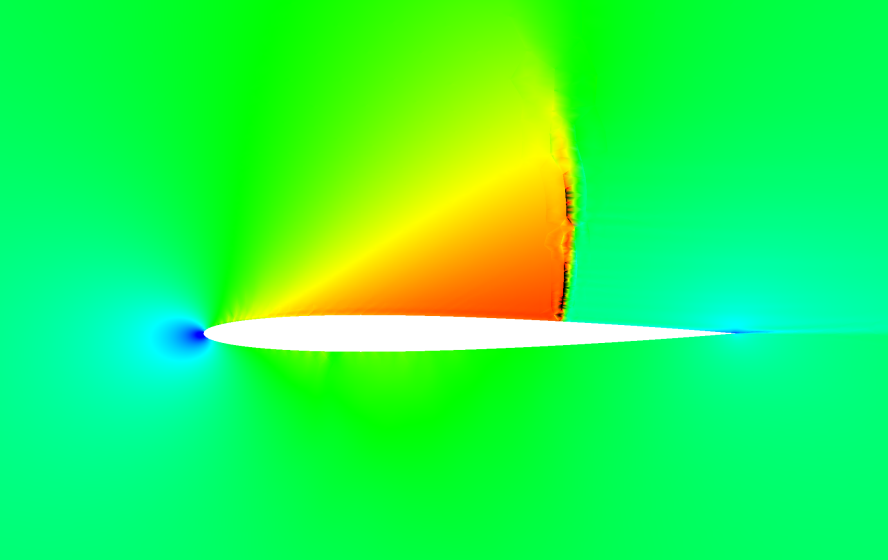
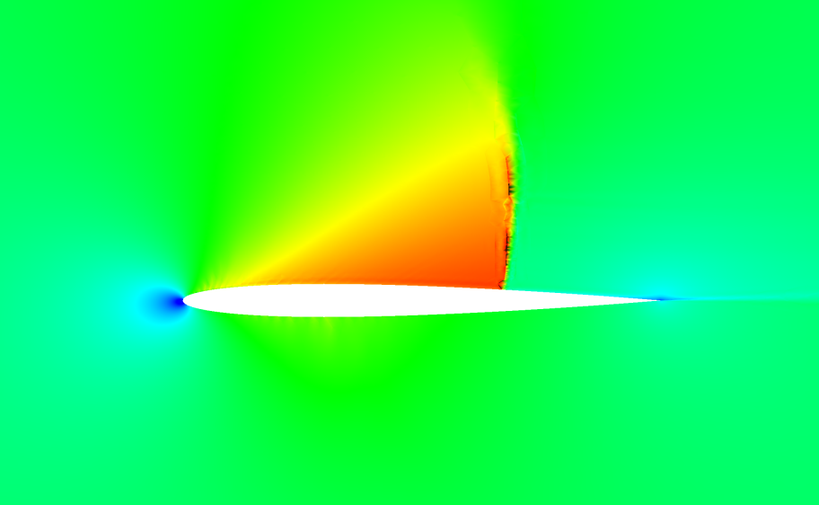
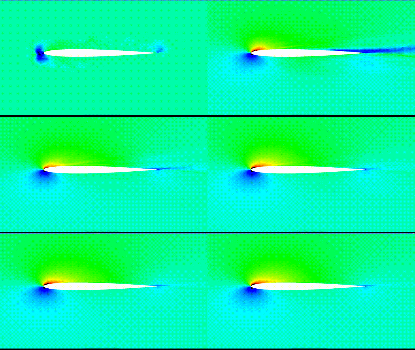
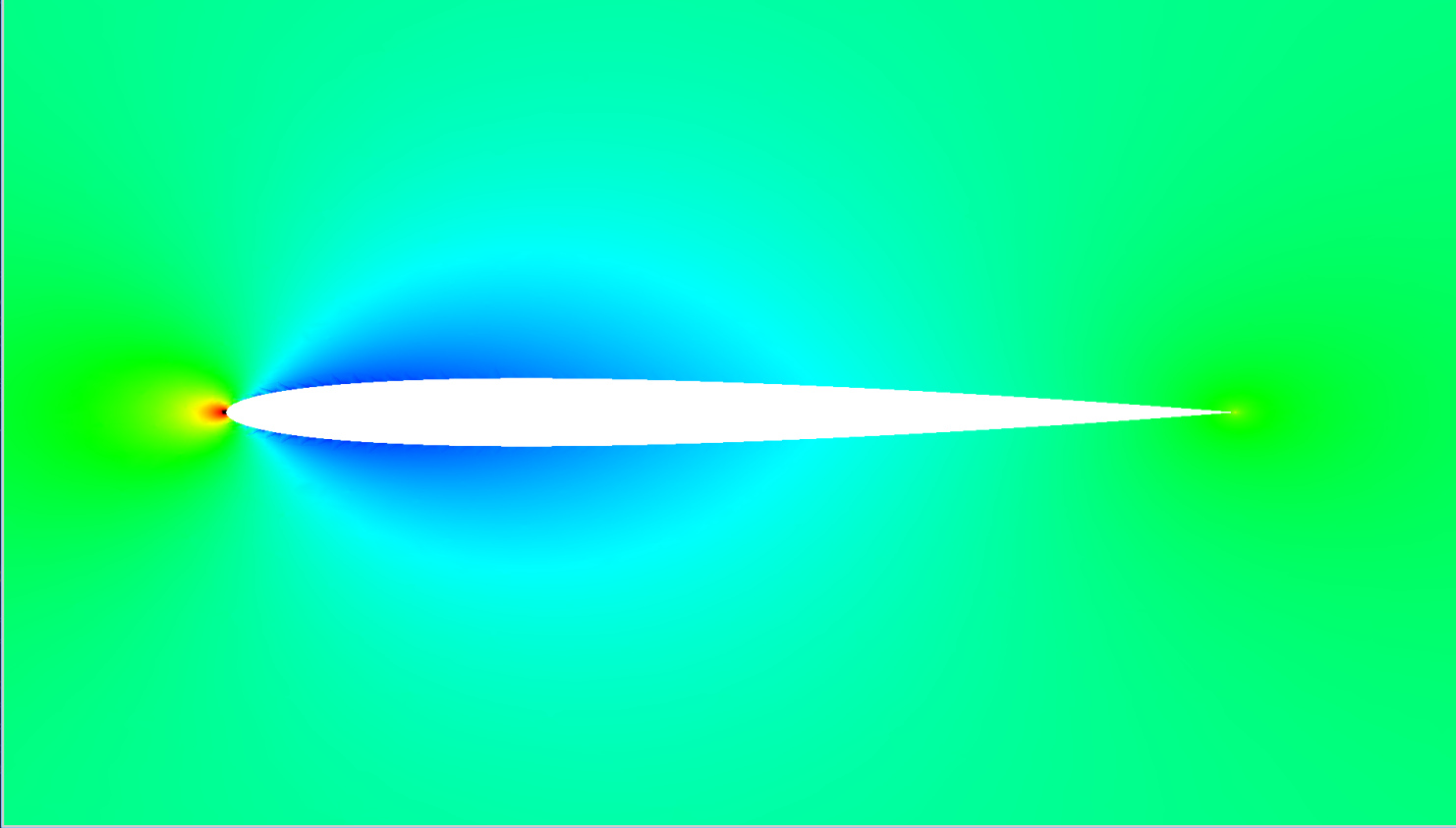
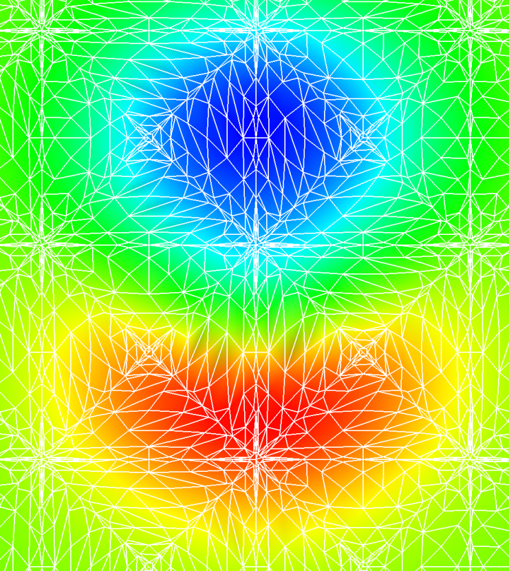
| NACA 0012 Airfoil at M=0.3, Alpha=6, Roe flux, Local Time Stepping | M=0.5, Alpha=0, Roe Flux, 1482 O(2) Elements, Converged |
|---|---|
 |
 |
| Density | X Momentum | Density |
|---|---|---|
 |
 |
 |
====
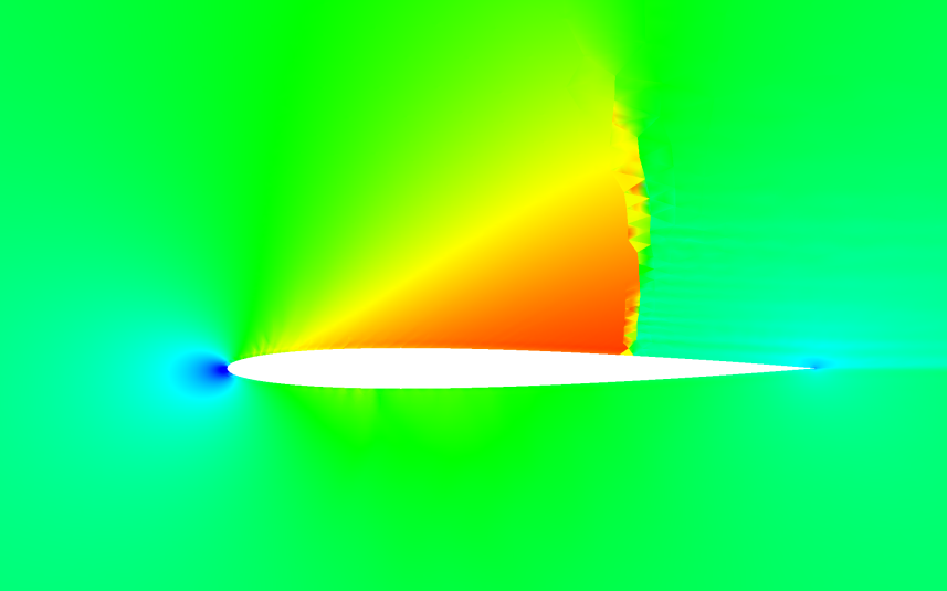
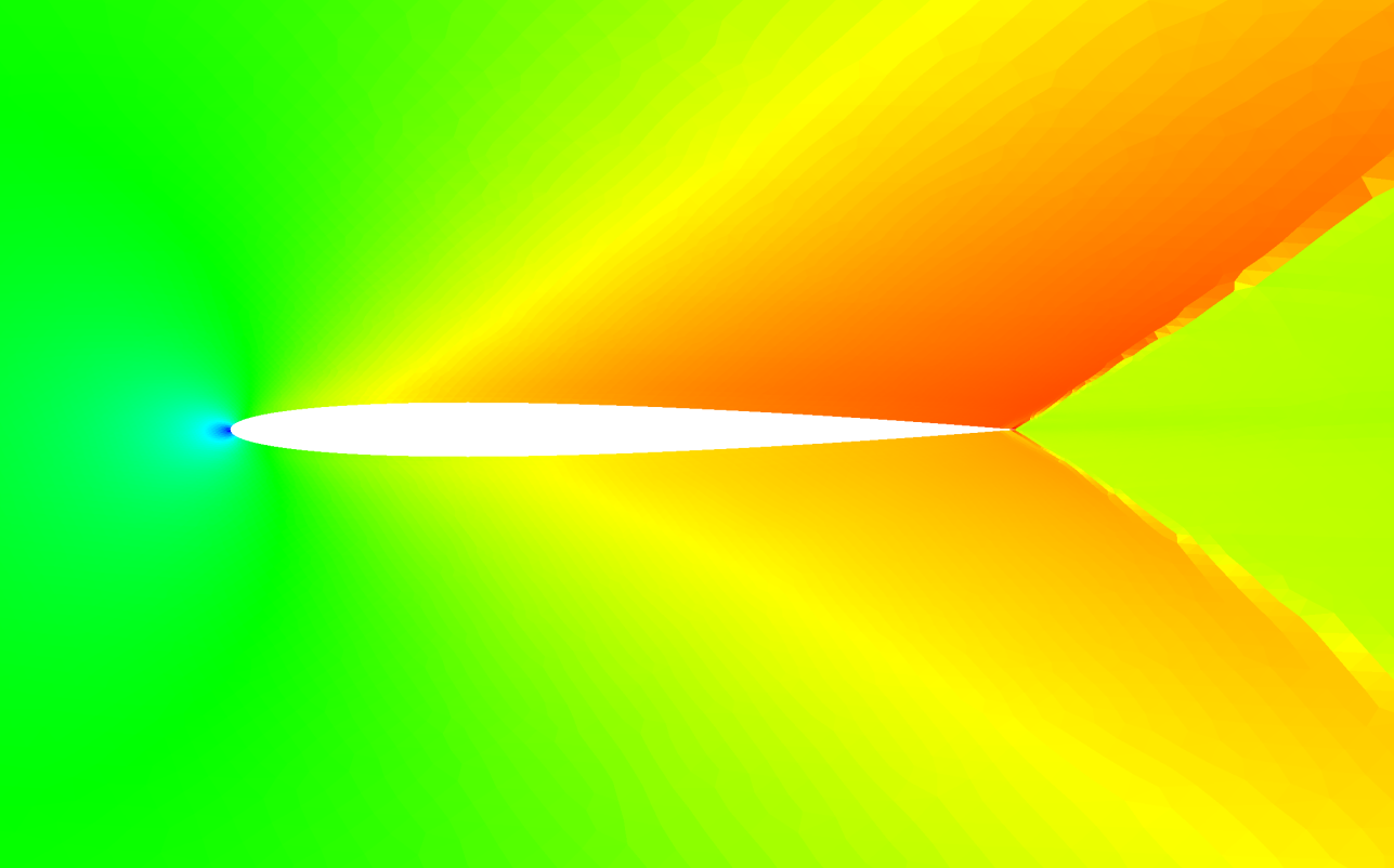
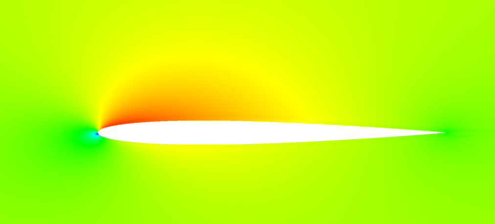
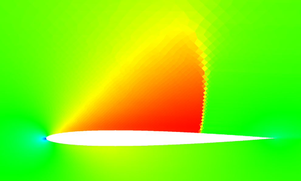
I've now continued testing and transonic cases are also working for P!=1. What's interesting now is that for P=0, the transonic solutions and shock tube solutions are wiggle free / monotone. Below is a transonic airfoil solution at Mach = 1.0 and 0.8, converged, on a mesh with 42,500 elements. The shock wave is finely resolved and is monotone. The convergence was also far more monotone and rapid than the higher order solutions.
The biggest difference between the 0th order solutions and higher order is the interpolation of the flux from the interior nodes. In the P=0 case, there is only one interior point and the flux is simply copied from the interior to the edge, as is typical of second order finite volume schemes. Reconstruction of the shared flux value at the edge is then handled via solving the 1D normal Riemann problem at the edge at first order. The resulting scheme should converge at 1st order, or P+1.
I think at this point, the wiggle problem I'm experiencing is due to the non-monotonicity of the interpolation of the flux. New extrema are being created, and my instinct is to eliminate the extrema by limiting the interpolated values to the min and max of the values in the interior. This would remove "extrapolation artifacts", but what is the impact on numerical accuracy?
| P=0, NACA 0012, Mach = 1.0, Alpha = 2, Interpolated Flux, Converged |
|---|
 |
| P=2, NACA 0012, Mach = 0.5, Alpha = 2, Interpolated Flux, Converged | P=0, Mach = 0.8, Fine Mesh, Converged |
|---|---|
 |
 |
Discontinuous Galerkin Method for solving systems of equations - CFD, CEM, ... hydrodynamics-fusion (simulate the Sun), etc!
- Jan S. Hesthaven and Tim Warburton for their excellent text "Nodal Discontinuous Galerkin Methods" (2007)
- J. Romero, K. Asthana and Antony Jameson for "A Simplified Formulation of the Flux Reconstruction Method" (2015) for the DFR approach with Raviart-Thomas elements
- Implement a complete 3D solver for unstructured CFD (and possibly MHD) using the Discontinuous Galerkin (DG) method
- Optimize for GPUs and groups of GPUs, taking advantage of the nature of the natural parallelism of DG methods
- Prove the accuracy of the CFD solver for predicting flows with turbulence, shear flows and strong temperature gradients
- Make the solver available for use as an open source tool
It is important to me that the code implementing the solver be as simple as possible so that it can be further developed and extended. There are other projects that have achieved some of the above, most notably the HiFiLES project, which has demonstrated high accuracy for turbulence problems and some transonic flows with shock waves and is open source. I personally find that C++ code is very difficult to understand due to the heavy usage of indirection and abstraction, which makes an already complex subject unnecessarily more difficult. I feel that the Go language makes it easier to develop straightforward, more easily understandable code paths, while providing similar if not equivalent optimality and higher development efficiency than C++.
I studied CFD in graduate school in 1987 and worked for Northrop for 10 years building and using CFD methods to design and debug airplanes and propulsion systems. During my time applying CFD, I had some great success and some notable failures in getting useful results from the CFD analysis. The most common theme in the failures: flows with thermal gradients, shear flows and vortices were handled very poorly by all known usable Finite Volume methods.
Then, last year (2019), I noticed there were some amazing looking results appearing on Youtube and elsewhere showing well resolved turbulent eddies and shear flows using this new "Discontinuous Galerkin Finite Elements" method...
Ensure you have the go language installed and in your path, then install prerequisites:
me@home:bash# sudo apt update
me@home:bash# sudo apt install libx11-dev libxi-dev libxcursor-dev libxrandr-dev libxinerama-dev mesa-common-dev libgl1-mesa-dev libxxf86vm-dev
me@home:bash# make
#### 1D shock tube test case
### without graphics:
me@home:bash# gocfd 1D

### with graphics:
me@home:bash# export DISPLAY=:0
me@home:bash# gocfd 1D -g

#### 2D airfoil test case
me@home:bash# gocfd 2D -F test_cases/Euler2D/naca_12/mesh/nacaAirfoil-base.su2 -I test_cases/Euler2D/naca_12/input-wall.yaml -g -z 0.08
If you are interested in reviewing the physics and how it is implemented, look through the code in "model_problems". Each file there implements one physics model or an additional numerical method for a model.
If you want to look at the math / matrix library implementation, take a look at the code in utils/matrix_extended.go and utils/vector_extended.go. I've implemented a chained operator syntax for operations that favors reuse / reduces copying and makes clear the dimensionality of the operands. It is far from perfect and complete, especially WRT value assignment and indexing, as I built the library to emulate and implement what was in the text and matlab, however it is functional / useful. The syntax is somewhat like RPN (reverse polish notation) in that you manage an accumulation of value over chained operations.
For example, the following line implements:
rhsE = - Dr * FluxH .* Rx ./ epsilon Dr is the "Derivative Matrix" and Rx is (1 / J), applying the transform of R to X, and epsilon is the metalic impedance, all applied to the Flux matrix:
RHSE = el.Dr.Mul(FluxH).ElMul(el.Rx).ElDiv(c.Epsilon).Scale(-1)
Update: [12/01/21]
I've implemented a min/max limiter that restricts values interpolated from the interior solution points to the edges in a couple of different variations. When the limiter is active, no interpolated edge values are higher or lower than the interior, All values used derive from the solution of the fluid equations in the interior nodes. This eliminates extrapolation overshoot at edges known as the Runge phenomenon. What I observed is that the Gibbs instability became more pronounced, with the "wiggles" appearing throughout the interior at higher frequencies, which confirms that the overall problem is actually in the interior polynomials, not the interpolation to the edges, or possibly a coupled version of the edge and interior.
I did find a description of a very similar project using the Flux Reconstruction method of Huynh Vandenhoeck and Lani, "Implicit High-Order Flux Reconstruction Solver for High-Speed Compressible Flows", which is a more complicated process with an identical resulting numerical scheme (on quadrilaterals/tenso product bases). Vandenhoeck notes that the Gibbs instability increases when the artificial viscoscity length scale is "too small", and in their case he reported that the length scale should be large enough to spread the shock over "a couple of cells" so as to avoid the instabilities inside the cell consequent from the intra-cell capture of the discontinuity.
I think the next step I'll take is to modify the artificial viscoscity to parameterize it similarly to Vandenhoeck, then run some experiments to validate stability when capturing shock waves over a couple of elements.
I've implemented interpolation of fluxes to the edges, replacing the interpolation of solution values followed by computation of the flux. It's currently an option for Lax and Roe fluxes. Below is a 2nd order converged solution using the new approach, showing very smooth solution contours.
It's definitely a more computationally expensive route, but it seems to be "correct", in that there are fewer interpolation errors evident in the solution. The results are substantially different in that we get:
- stable and convergent solutions at subsonic Mach for orders 0,2,4, unstable at P=1, likely due to interpolation overshoot
- smoother and more realistic solution contours without the edge defects
I think it's likely this is a better formulation for the edge computations, but we need something that will eliminate the spurious new minima/maxima being introduced by the flux interpolation. TVD/ENO concepts come to mind, where we limit the interpolated values so as not to introduce new minima/maxima, but I think it's important to formulate such an operation so that it doesn't create aphysical effects, especially in the time accurate solver.
New theory: it's the interpolation of the solution values to the edges that is the culprit - instead, I'll interpolate the flux from the solution points to the edge along with the solution values, then compose the Roe flux as an average of the interpolated L/R fluxes plus terms arising from the interpolated solution values for the Riemann problem at the edge.
| NACA0012 M=0.8, AOA=2 New RT Element vs Lagrange Basis vs Jacobi Basis |
|---|
| L2 Convergence Compared |
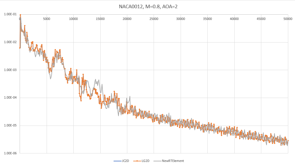 |
Update [11/15/21]: The results are in - a completely new Raviart-Thomas element design is now available, and it gives results that are very similar to the prior implementation. It's hard to judge which is superior, but at this point the new basis requires a slightly higher artificial dissipation for the airfoil case and seems to achieve similar convergence rates. The "wiggles" in the shock tube case are still present. Mostly, I'd say the results prove that the RT element basis is not responsible for the general instability with shocks. The "good news" here - after re-designing and replacing the core of the DFR method, we get very similar results, which gives new confidence that the DFR core is likely correct. New theory: it's the interpolation of the solution values to the edges that is the culprit - instead, I'll interpolate the flux from the solution points to the edge along with the solution values, then compose the Roe flux as an average of the interpolated L/R fluxes plus terms arising from the interpolated solution values for the Riemann problem at the edge.
I see a/the problem now! The current build of the RT element used for divergence is incorrect, or at least is different
from other constructions in a fundamental way. There are two polynomial domains included in the RT element, one is a
2D vector polynomial field [Pk]^2, and the other is a 2D scalar polynomial multiplied by the vector location
[X](Pk). These are allocated to the interior points and to the edges separately.
I had chosen to use a 2D polynomial basis of degree "P", the same degree as the RT element to implement the basis functions for edges and interior. I multiplied the edge functions by [X] and used the highest order basis functions for the edges, left over after consuming basis for the interior points.
Now, after reviewing V.J. Ervin, "Computational Bases for RTk and BDMk on Triangles, I believe the RT element basis he constructed is superior and that mine likely has some asymmetries that may be producing the "wiggles".
I'm now working on a revised RT element basis, following Ervin's design.
Next: I'm going to look into an exponential filter for the polynomial interpolation to the edges.
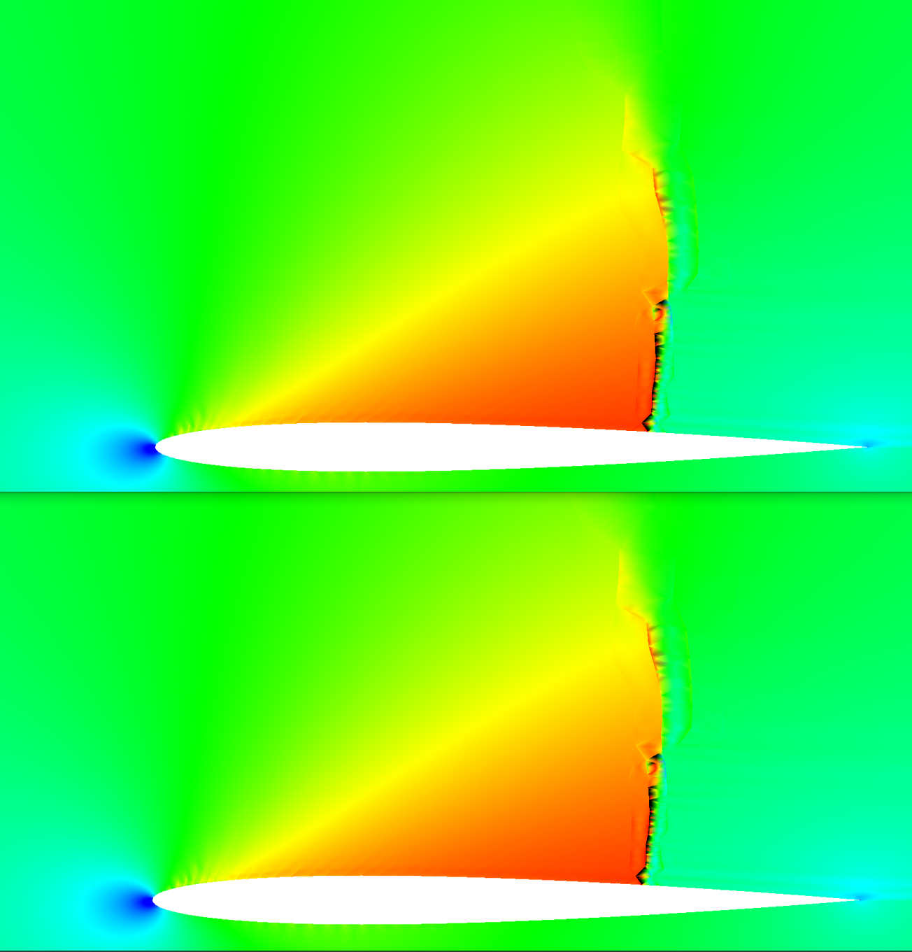
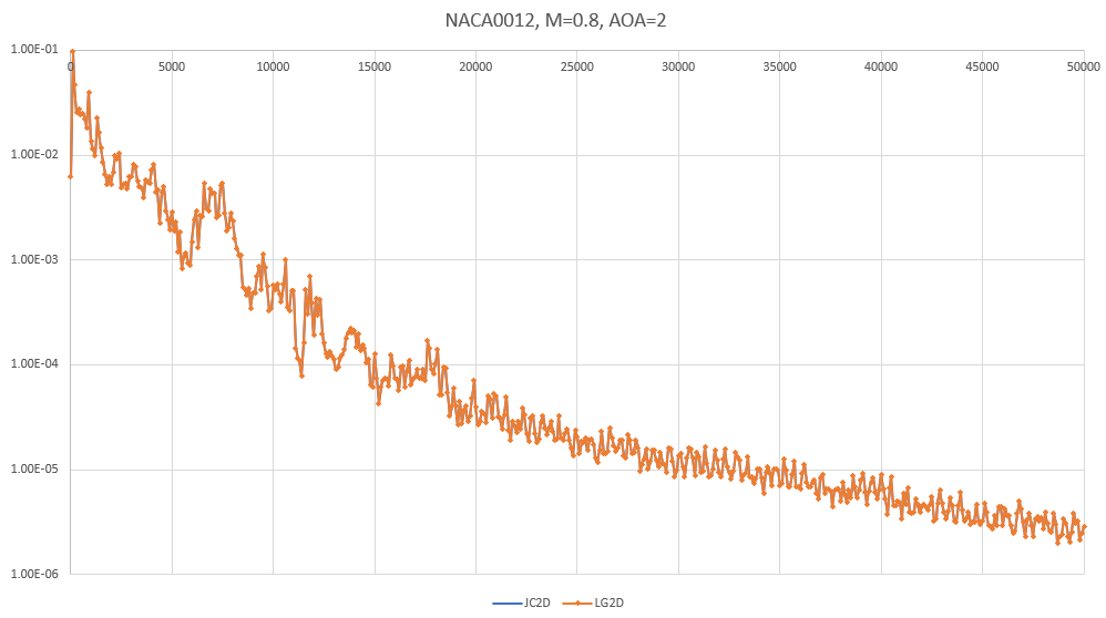
I've implemented a "true" 2D Lagrange polynomial basis for the scheme and now can compare results using the Jacobi Orthonormal 2D basis with the Lagrange 2D basis. Below are two cases run at second order, one using the Jacobi and the other the Lagrange basis - they basically overplot each other, both in convergence history and in the final Mach number distributions.
Looking into this a bit - the Interpolation matrices for each basis are identical, as expected. As a result, the interpolation from the solution nodes to the edges is the same between the two. The basis used for the divergence within the RT element is different between the two, but that seems to not impact the results.
My conclusion based on this experiment: The interpolation to the edges appears to be more important to the solution than the polynomial basis used in computing the divergence.
| NACA0012 M=0.8, AOA=2 Lagrange vs Jacobi Basis | L2 Norm Convergence History |
|---|---|
| Mach Number | Convergence, CFL = 3, Kappa = 3 (Artificial Dissipation) |
 |
 |
After fixing up the limiter and the epsilon artificial dissipation and doing some numerical studies with the shock tube and airfoil, I'm convinced that the core flux/divergence scheme is a bit too "bouncy" as compared with other schemes. The main issue with the limiter now is that there is "buzzing" around the shock wave, where the shock bounces back and forth between neighoring cells, which stops convergence. There's one more thing I can do to make the limiter work better, by filtering on characteristic variables instead of the conserved variables. This has been shown to focus the limiting more where it's needed, and delivers a much cleaner result with less dissipation. I'll definitely implement that later, but I think it's time for some core work first.
Given the success that Jameson and Romero experienced with their simplified DFR and when compared to the other DFR results, it seems this current method is not as able to handle shock waves without significant Gauss instabilities. This has become more clear when using the artificial dissipation approach, which captures shock waves within a single element, an excellent feature that works now within this method. While in-element shock capturing works now, there are aphysical extrema within the shock containing cells that Persson, et al did not experience. There are many excellent results with the method so far, and it does seem close to complete and capable, so my question is: how can the current method core be improved to fundamentally be better at handling shock waves?
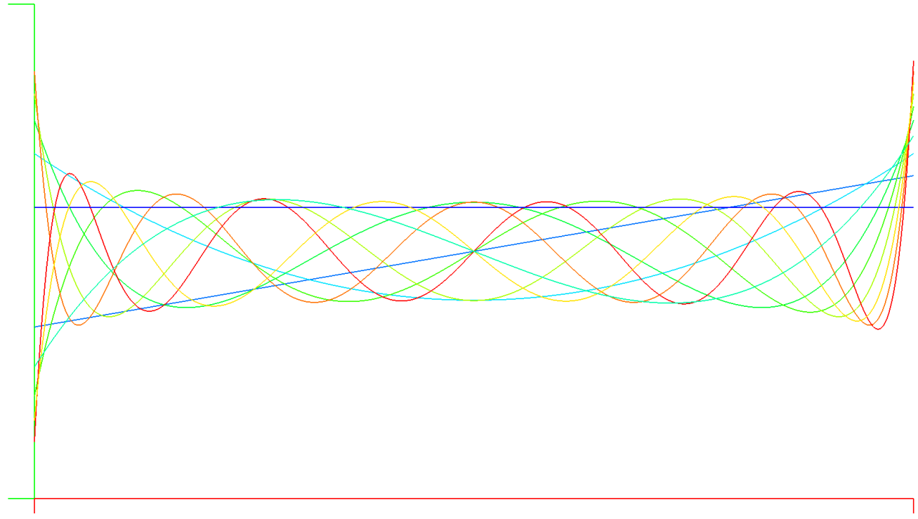
After thinking about the above question, I think the answer may lie in the basis functions I've been using. The basis functions define the modes energy has access to within the element, with various wave shapes that store energy. Though Romero and Jameson used Lagrange Interpolating polynomials as their basis, I chose to use the Jacobi polynomials in a tensor product as Hesthaven does in the book I've used for the core of this method. Basis functions have different levels of variance from their mean, and my concern is that the Jacobi polynomials may be too "wild" when interpolating to the element's extrema - specifically the interpolation of solution values to the edges.
| Jacobi Polynomials to N=9 | Interval: -1 < X < 1 |
|---|---|
| Alpha = Beta = 0 | Alpha = Beta = -0.99 |
 |
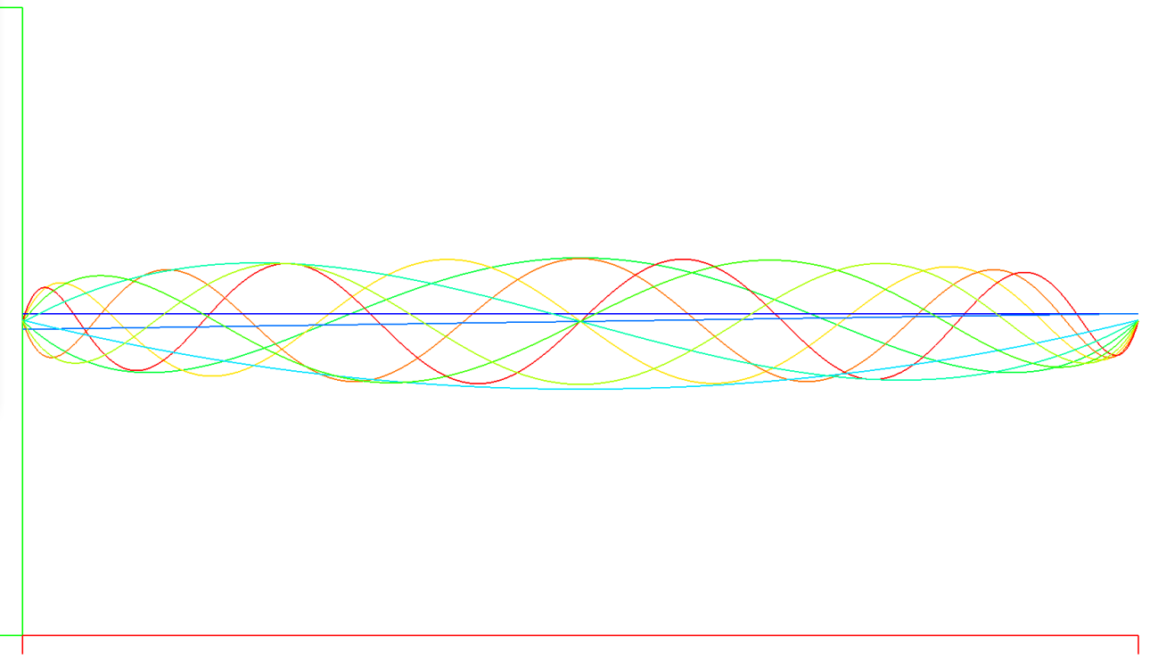 |
In the above plot of the Jacobi polynomial in the interval -1 to 1, we can see what appears to be a collapse in the values of the polynomials of all orders at the extrema of the interval. Intuition says we want to have all modes equally available across the interval, and when we use the Alpha and Beta parameters to stretch the polynomials we can improve the collapse as see in the plot on the right, although there is still quite a narrowing among modes. I tried running the airfoil case using the basis on the right and it does seem to improve both convergence and extrema, but only marginally.
Up next: I'm implementing Lagrange Interpolating basis functions to the finite element construction as an alternative. This will allow for comparison among basis functions and selection of the best for shock waves.
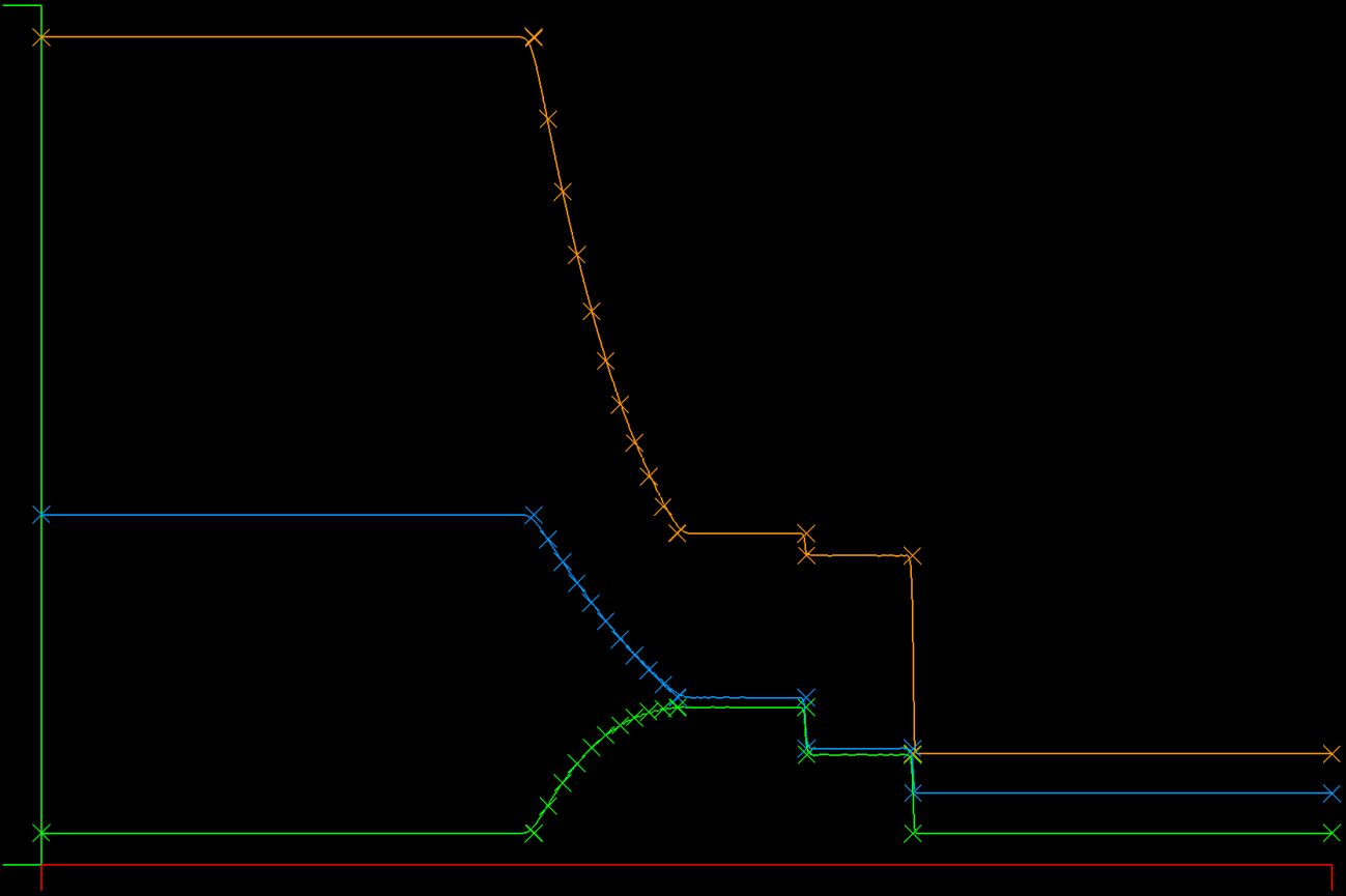
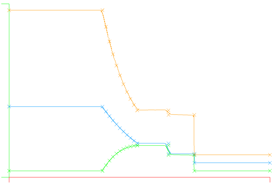
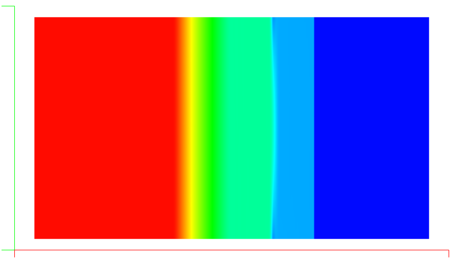
I've replaced the previous broken Runge Kutta time advancement scheme with an explicit SSP54 scheme from Gottlieb, et. al. and now the SOD shocktube results are in excellent agreement with the exact result as shown below. Note the slight bulge in the density profile at the centerline - or alternately it's a lag near the tube walls.
| SSP54 Time integration Centerline Compared with Exact Solution | Density in 2D |
|---|---|
 |
 |
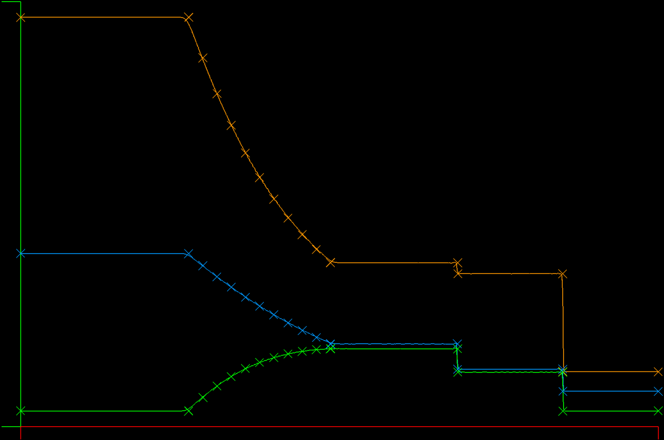
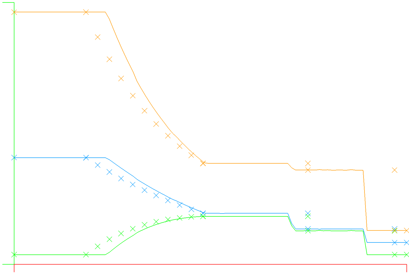
Previously: Good news: the source of the bug is clearly the time integration (Runge Kutta 4th Order SSP algorithm) - simply changing one of the constants from 0.25 to 0.4 fixes the wavespeed issue completely. I'll revisit the implementation once I find out where I got the coefficients from - in this case I haven't included their source reference in the code (DOH!)
| Centerline Compared with Exact Solution | Density in 2D |
|---|---|
 |
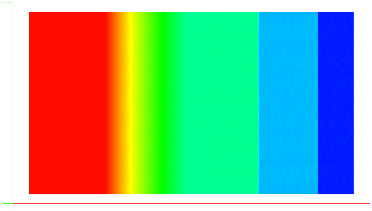 |
I've implemented a 2D version of the 1D shock tube with graphics and the exact solution for comparison.
In the above snapshot, we can see that the shock wave and all waves are running at incorrect wave speed, indicating there is a bug in the physics of the solver somewhere. This is actually good news in that I can hope the general instabilities around shock capturing could be solved by fixing this bug!
So far I've verified the bug exists with both Lax / Rusanov and Roe numerical fluxes, and is the same at 100 points resolution and 500 points.
On the bright side, we see the sharp resolution of the shock wave and near perfect symmetry in the solution, so we just need to chase down the wavespeed error in the solver physics.
I've implemented two different gradient calculations to compute the dissipation and verified they function correctly.
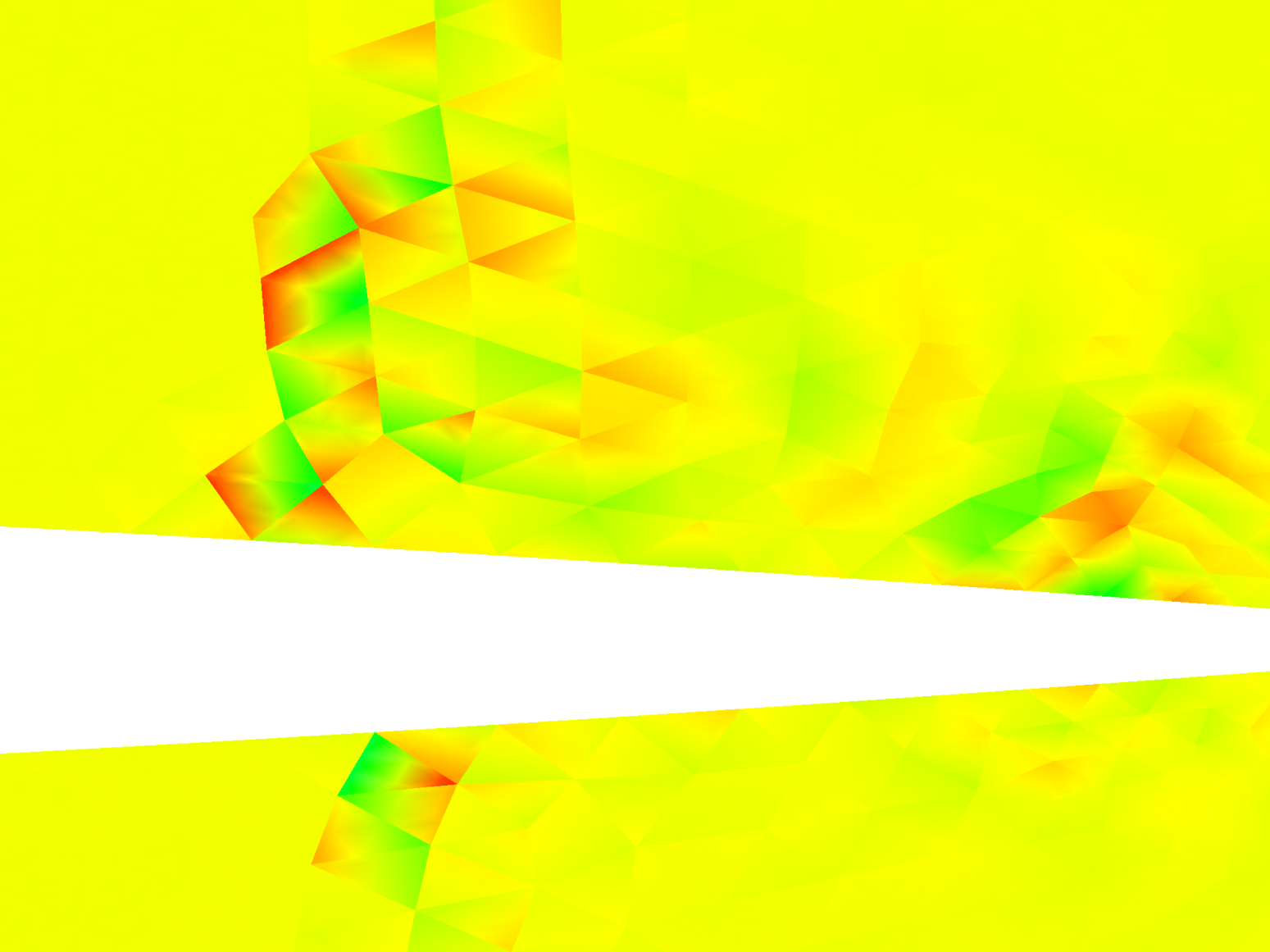
The dissipation is not able to suppress shock induced (Gibbs) oscillations as implemented, and I think it's clear that this is due to an effect described by Persson involving the continuity of the gradient operator. In the picture below (2nd order, Roe flux, M=0.8), you can see the base of the shock wave above the NACA0012 airfoil. As the shock strengthens, the X derivative of X momentum is growing and clearly is discontinuous between elements, despite being computed from a C0 continuous X momentum field (accomplished using the RT element). In order for the sub-element shock capturing to work properly, Persson suggests that the gradient must be smooth across elements, otherwise the jumps between elements are strengthened instead of being diminished as needed. The solution described is to use the "LDG" method for computing 2nd order derivatives as described by Cockburn and Shu in 1999.
Next, I plan to implement 2nd order derivative continuity along the lines of the LDG method, which will also support the next steps in implementation of viscous equations (Navier Stokes). Hopefully, we'll kill two birds with one stone: sharp shock capturing at high order accuracy and viscous solutions!
I've implemented laplacian artificial dissipation that tracks shock induced instabilities using the Lagrangian solution element to compute the flux derivatives and also for the divergence of the dissipation field. The method works well for 1st order calculations, with sharp shock resolution and fast convergence, though the intra-element shock resolution is marked with a significant discontinuity with the edges of the shock capturing cell. When the shock aligns with the edge, the result is a near perfect shock capture, but when the shock is not on the edge, the intra-cell solution has spurious internal oscillations.
Based on these results, I'm implementing what seems a simpler and more appropriate method: The dissipation flux will be calculated for all points within the Raviart Thomas element used for the calculation of the fluid flux divergence. The resulting dissipation flux [epsR, epsS] is then added to the physical fluid flux [fluxR,fluxS] and then the divergence of the combined flux is calculated using the RT element divergence operator. I'm anticipating that this approach should provide added stability to the flux field, which is an (N+1)th order polynomial field that overlays the (N)th order solution field. In the prior approach, the (N)th order divergence of the artificial dissipation is added to the (N+1)th order derived physical divergence, and I think that is creating aliasing errors that are unstable.
Update: I finished the shock finder, below is a plot of the "ShockFunction" (function 100) for the NACA0012 airfoil at M=0.8 on it's way to becoming unstable. We can clearly see the shock function has picked up instability at the forming shock wave on the trailing edge and at the curvature inflection on the top. We can also see the shock indicator tracking the startup transient wave coming from the leading edge. It looks to be very effective, as reported! Next step - implement dissipation for "troubled elements" to remove the instability.
After some research, I found a general pattern and one excellent summary from Persson, et al describing how to capture shocks within the elements themselves while eliminating the aliasing oscillations.
Persson and Peraire demonstrated the following approach:
- Isolate elements that are experiencing shock instability with a "shock finder"
- Implement dissipation within only those elements to remove the unstable modes
For (1), they use the fact that in a smooth solution, the energy dissipates rapidly as the expansion order increases. They form a moment, or inner product across each element that evaluates how much energy is present in the last expansion mode as a ratio of total solution energy. Where this ratio exceeds a threshold, it indicates a lack of smoothness that identifies where the "fix" is needed.
I'm currently working on calculating the shock finder from Persson, after which there are a variety of dissipation and/or filtering approaches we can use, for instance the modified Barth / Jesperson filter used by Zhiqiang He, et al.
Update: The data are in - the new Roe-ER flux is faster to compute and has good characteristics, so it's a good thing and will be useful for turbulence capturing and strong shock applications later. However, tests showed that using either Roe or Roe-ER flux calculations crashed due to odd-even instability with shocks past maybe Mach 0.6 on the airfoil test. I'm thinking that we need to stabilize the flux at the border of the element using higher order approximations and clipping them using MUSCL/TVD approach. This is similar to a typical J->J+1 structured approach but using "wiggle simulation" for the flux derivatives at the boundary. I wonder also if I'll need to increase the derivative degree at the boundary along with the overall order of the element? It's very do-able, though I think I'd want to do a more analytic derivation for sampling higher order fields within elements.
Removing the "wiggles", part X: There are still odd-even instability modes being triggered by shocks, which for now I'm assuming are being introduced by the flux transfers between elements. It's possible that the discontinuities from shocks are landing in the polynomial basis and amplifying there, but first I'm going to eliminate the flux transfer amplifications before doing anything inside the element.
I'm planning now to implement a TVD scheme at 2nd order for the flux transfer as follows:
- Interpolate the Q field to the edge using the element polynomial basis (same as now)
- Interpolate an additional value close to the edge, say 0.01 of the edge length close
- Use the two values on either side of each edge to construct a MUSCL with TVD to obtain the edge flux
This approach should introduce damping to oscillatory modes crossing the boundary, while slightly improving the accuracy of the interpolated flux.
Working on an enhanced flux transfer scheme that promises to protect against odd-even decoupling ("wiggles") while minimizing artificial dissipation that can destroy turbulence fields, etc.
The scheme I've located is by Xue-Song Li, et al from an AIAA paper in 2020, who described the "Roe-ER" flux, which combines features of the Harten entropy fix and the rotated Roe flux schemes. It looks very efficient and in the papers it seems to do a very good job at the wiggle issue while delivering excellent accuracy.
My remaining concern / question is about whether the use of a flux limiter for transfer of flux at the element faces is sufficient to damp oscillations, or whether I'll have to couple elements more deeply, thus removing a principal advantage of Nodal Galerkin methods - that of "compact support". We'll soon see!
Working on adding routines to invert and solve block matrix systems so that I can implement an implicit time advancement scheme.
Implicit fluid dynamics schemes all use the flux jacobian of the underlying equations, which yields a system of equations that has "blocks" consisting of the 4x4 (2D) or 5x5 (3D) matrices representing each nodal point. This requires that we have a way to invert the system matrix, or use a solver approach to get the final update in the time advancement scheme.
The work I'm doing now will add a capability to efficiently store the full block system matrix and use it to solve for the time update.
Investigating algorithmic methods to speed up convergence to a steady state solution. These techniques can also be applied to unsteady/time varying solutions by solving incremental time advancement sub-problems.
There are many algorithms in the literature, including:
Implicit time advancement within each element, which should improve the convergence rate as the order of the elements increase.
Improves global implicitness by solving advancing lines(2D) or planes(3D) through the field. This technique has been shown to greatly improve convergence of viscous problems with cells packed tightly to surface geometry.
Propagates low frequency changes rapidly through the finest mesh using nested coarse meshes.
Used to remove stiffness in propagating high frequency changes where the difference in wave speeds is large. Examples include very low speed flows where the acoustic wave speed and sonic wave speeds differ greatly, or viscous problems where the viscous eigenvalues are very small compared to sonic waves.
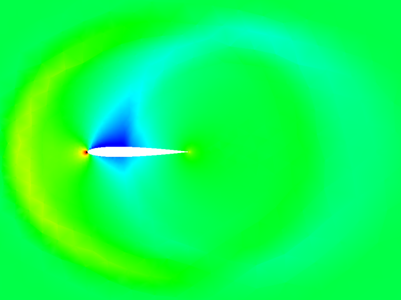
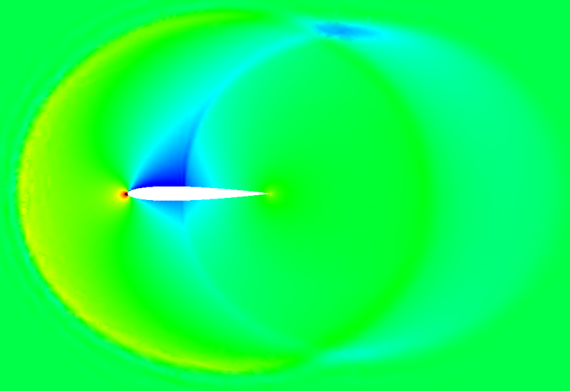
Time Accurate Abrupt Start Transients
| 1st Order | 4th Order | 5th Order |
|---|---|---|
 |
 |
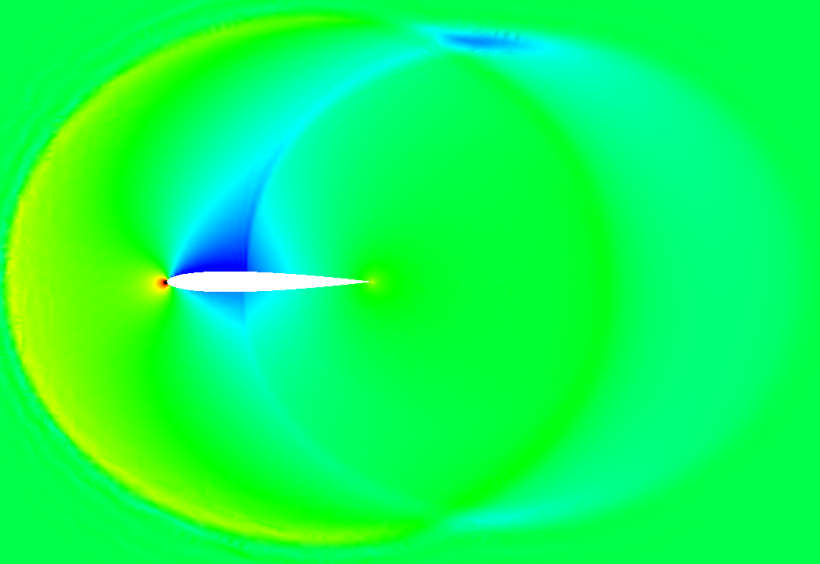 |
The above is just for fun - the wave interactions are all subsonic with Minf = 0.5 and AOA = 2. It's interesting to compare the resolution of the fine wave interactions between the different polynomial orders.
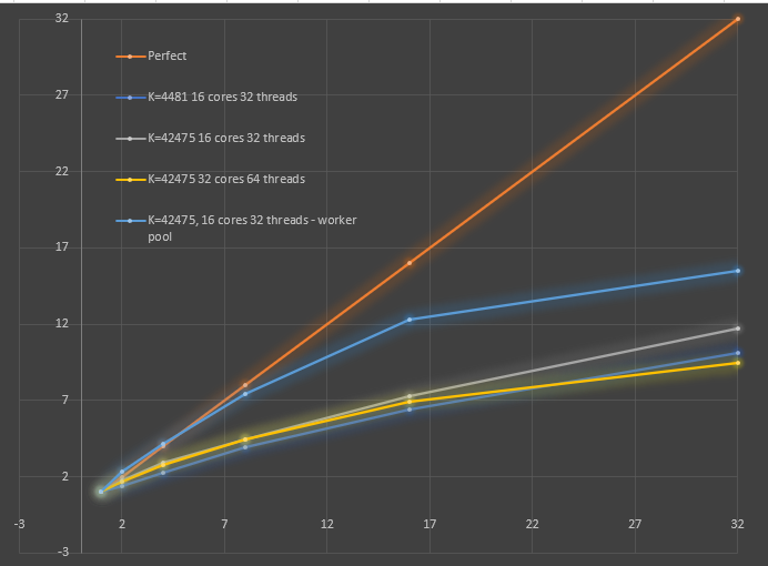
Improved parallelism - Time step and edge flux computations are now computed within a worker pool, which minimizes the thread start/stop overhead. I improved the cache locality by grouping edges with a given primary element number into the same group. Finally, I measured the optimal number of elements per core for best cache locality, and used that to automatically set the number of goroutines used for a given problem. The resulting parallelism is shown in the below graph
I measured the instruction rate and on the 16 core AMD Threadripper server, we're doing about 1.3 Giga-ops/second on 32 threads. Note however that each instruction can be a packed SSE or other multi-instruction like vectors, so this is not equal to the FLOPS count. To obtain the FLOPS, I'll have to count the individual types of instructions and multiply that by the number of operands per each instruction. I think it's likely we're doing about 4x the above in terms of FLOPS, so we're in the 4-5 GFlops range, but I can't be sure until doing the full count.
A very likely reason for the scaling fall-off is the limited memory bandwidth of the AMD threadripper servers, one a 1950X and the larger is a 2990WX. The memory bandwidth of the 16-core 1950X is is 50 GB/s, which translates to a limit of 3.1 GFlops for non-cache local workloads: 3.125 Gops/s = 50 GB/s / 8-bytes per operand / 2 load and store operations per operand, so the observed 1.3 could be hitting close to the limit when multiplied by the operands per operation, say 2x if they were all AVX SIMD operations, which is the limit of the 128-bit SIMD register on this AMD Threadripper. Another contributing data point: the 2990WX runs out of parallel scaling much earlier than the smaller server, and the explanation is that it has a problematic memory architecture: 16 cores of the 32 total have to have memory accessed remotely through the other 16. This effectively limits the memory bandwidth to 64 GB/s, which is hardly more than the smaller machine. This would explain the steeper falloff on the 2990WX.
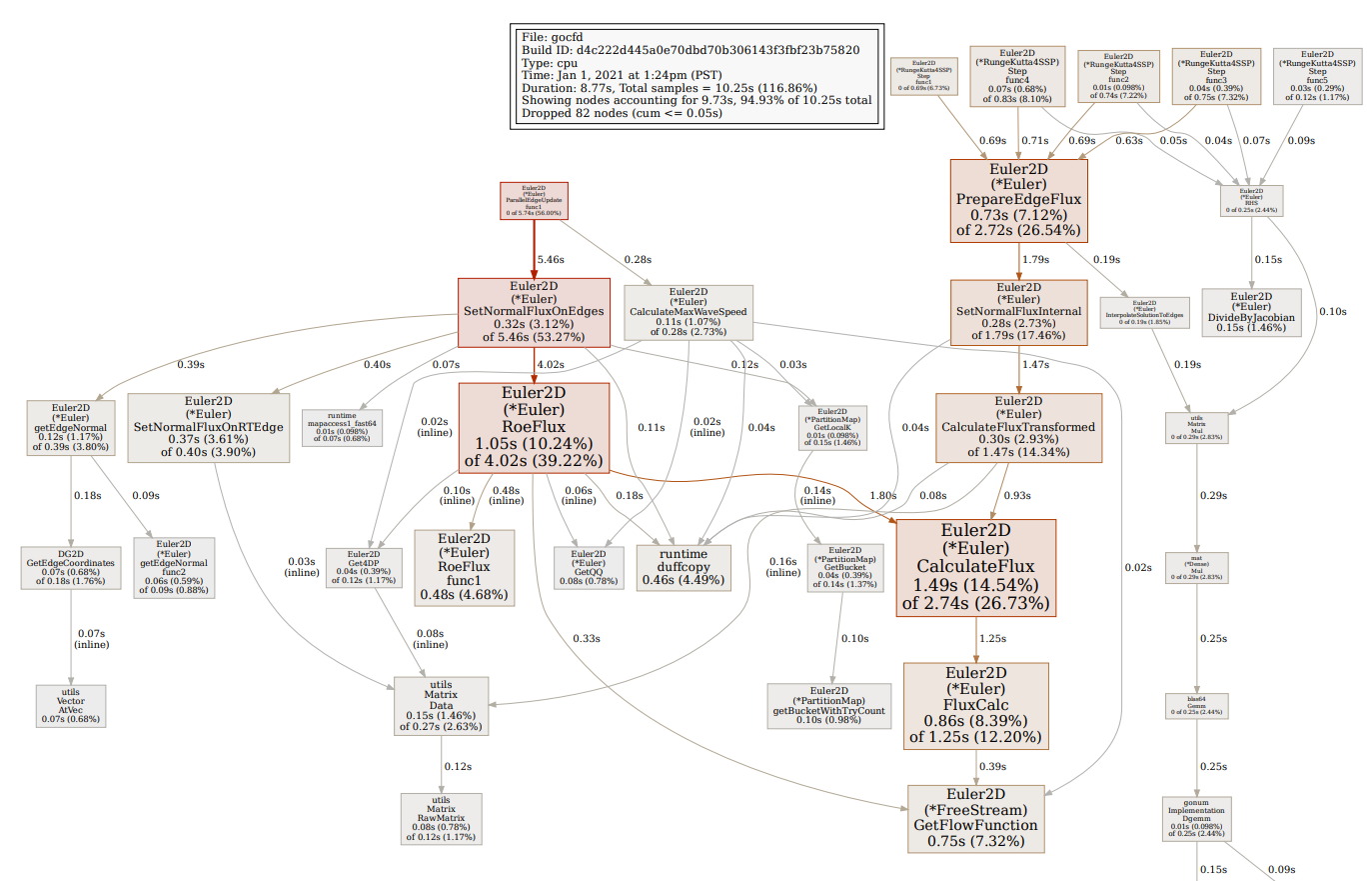
I added a command line option to generate a runtime profile for only the solver portion of the code, for example, this command:
gocfd 2D -I input-bench.yaml -F mesh/naca12_2d-medium-lal.su2 -s 100 -p 1 --profile
The above command will run a 2D case with the residual progress printed every 100 steps using one processor, and will output a runtime profile that can be used to generate a PDF like this using go tool pprof --pdf /tmp/profile354612347/cpu.pprof:
At this point, the runtime profile is pretty flat and clean of excess memory allocation. One helper function sticks out - GetQQ() - which reshapes various solution vectors into a more convenient shape. It's always a bad idea to mutate and copy data around in the performance pipeline - this is an example at 0.8% of the runtime. Another bad helper function is Get4DP, which gets pointers to the underlying data slices in various matrices - it's using over 1% of the overall time. Most of the usage of Get4DP applies to matrices that will never actually be used as matrices anyway, which is annoying and could be easily fixed by just not using matrices at all for those. One more: PartitionMap.GetBucket is using 1.4% of runtime, and all it's doing is retrieving which parallel bucket we need from the map using an iterative algorithm guaranteed to use at most 1 iteration. This is a consequence of the load balancing algorithm I've implemented that is not directly invertable - could improve that somehow. Overall, there's a handful of overhead totalling maybe 5% immediately apparent.
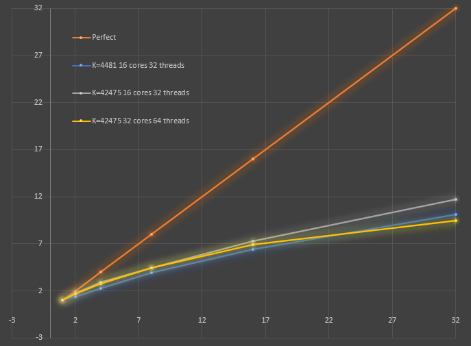
The above graph shows parallel CPU scaling for two meshes, one coarse (K=4,481) and one fine (K=42,475) on two different multi-processor Linux servers, each an AMD threadripper architecture from 2018/19. On the 16 core, 32 hyper-thread machine, we get a max scaling of around 12x on 32 threads, and we might expect to see scaling to around 20x on 32 hyperthreads if we were perfect (a hyper-thread is not equivalent to a core). Interestingly, on the machine with twice the CPU cores, we see slightly worse scaling, especially at higher parallelism request. Because of this second finding, I believe we are seeing performance degradation due to cache conflicts, where the processors are unable to happily share access to the cache because of cache contention. I've been anticipating this effect, as I've organized the memory accesses in ways that might trigger a lot of strided accesses that may not be cache friendly, which will incur this kind of effect on an SMP system. More investigation is needed to determine what is causing the apparent contention...
New Year's Day progress!
I partitioned the 2D solver by elements for enhanced parallelism. The solver now computes the RHS and time stepping fully parallel, but must still synchronize between each time sub-step (within the Runge-Kutta solver) to exchange data at edges, which is also done in parallel. So there are now two discrete stages/types of parallelism, one for the full domain of elements, and one for the edge exchanges and flux computation.
As a result of the partitioning, the parallelism is far better and we can get much faster solution times. The level of parallelism is well suited to machines with less than 100 processors. For more parallelism, we will need to use a mesh partitioning algorithm that selects the element partitions so as to minimize the surface area shared between partitions, such as the commonly used tool "metis". When the elements are partitioned in that way, we can isolate the time spent in synchronization to exactly the minimum necessary. By comparison, now we're doing all edge flux computation during the synchronization period.
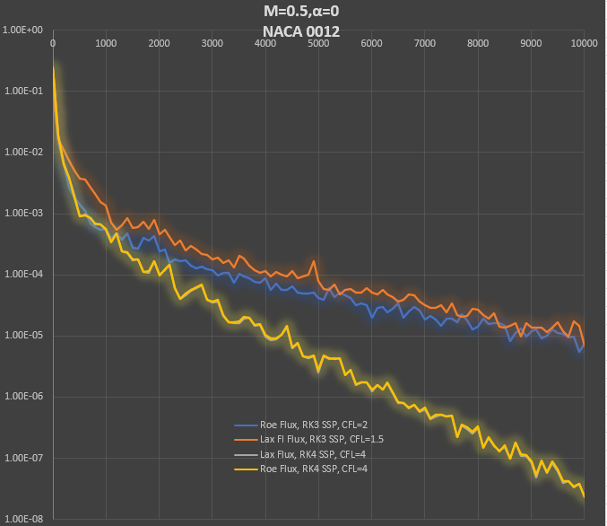
In the graph we compare convergence to steady state using two kinds of flux calculation and two types of Runge Kutta time advancement. The RK4 SSP time advancement is far superior in terms of CFL stability, as expected, without much increase in computational work or storage as compared with the RK3 method. The difference between the interpolated flux and the normal (interpolated Q, then calculate flux) is very small. The Lax and Roe flux results with RK4 are almost identical, the two lines on the graph are indistinguishable.
A lot of progress across a number of areas this week:
- Time advancement scheme - RK4 SSP in place of RK3 SSP, big stability and speed improvement with CFL now up to 4 (was 2) on NACA 0012 test cases
- Experiments with direct interpolation of Flux to edges in place of interpolation of conserved variables and calculation of flux -- did not appear to improve odd-even oscillations or higher order stability -- only tested on Lax flux, as current Roe flux would need extensive changes to implement
- Convergence acceleration for steady state problems - local time stepping
- Experiments with transonic flow with moderate shocks over airfoils -- Odd-even oscilations pollute the solution when there are shock waves and cause fatal instability for the Roe flux, although the Roe Flux is the original Roe flux, which has known issues with odd-even oscillation stability
As a result of the above experiments, the next focus is on:
- Solution filtering with shock/discontinuity detection
- Must be compatible with higher order methods and allow high order fields with shocks without destroying the high order capture -- I found a promising compact WENO filtering scheme designed for high order Galerkin type methods, paper here
- Multigrid convergence acceleration
- A complication: normal multigrid methods use agglomeration to compose the lower order meshes from the fine mesh. Currently, we only have triangular elements, so we can not use quad or other polygons that arise from agglomeration.
- A possible solution: compose RT and Lagrange elements for quads and polygons to enable later use in Navier-Stokes and multigrid
The solver now uses multiple cores / CPUs to speed things up. The speedup is somewhat limited, I'm currently getting about 6x speedup on a 16 core machine, but it was very short work to get this level of speedup (a couple of hours). The face computations are parallelized very efficiently, and the same approach and structure should be fine to scale to thousands of cores.
The shortcoming of the current parallelism is that it uses only 4 processes to handle the heavy compute matrix multiplications, so about half of the computation is only getting four cores applied to it. The number 4 comes from the number of 2D Euler equations (mass, x,y momentum and energy = 4 equations). I could improve the speedup drastically by re-arranging the core to accept partitioned meshes, but in 2D I think that might be overkill. The 3D solver will absolutely be built to do parallelism this way, so that we can use 1000 core architectures, like GPUs. I did parallelize the matrix multiplication directly, but the overhead is too high without more aggressive memory re-use work, which would begin to make the code ugly.
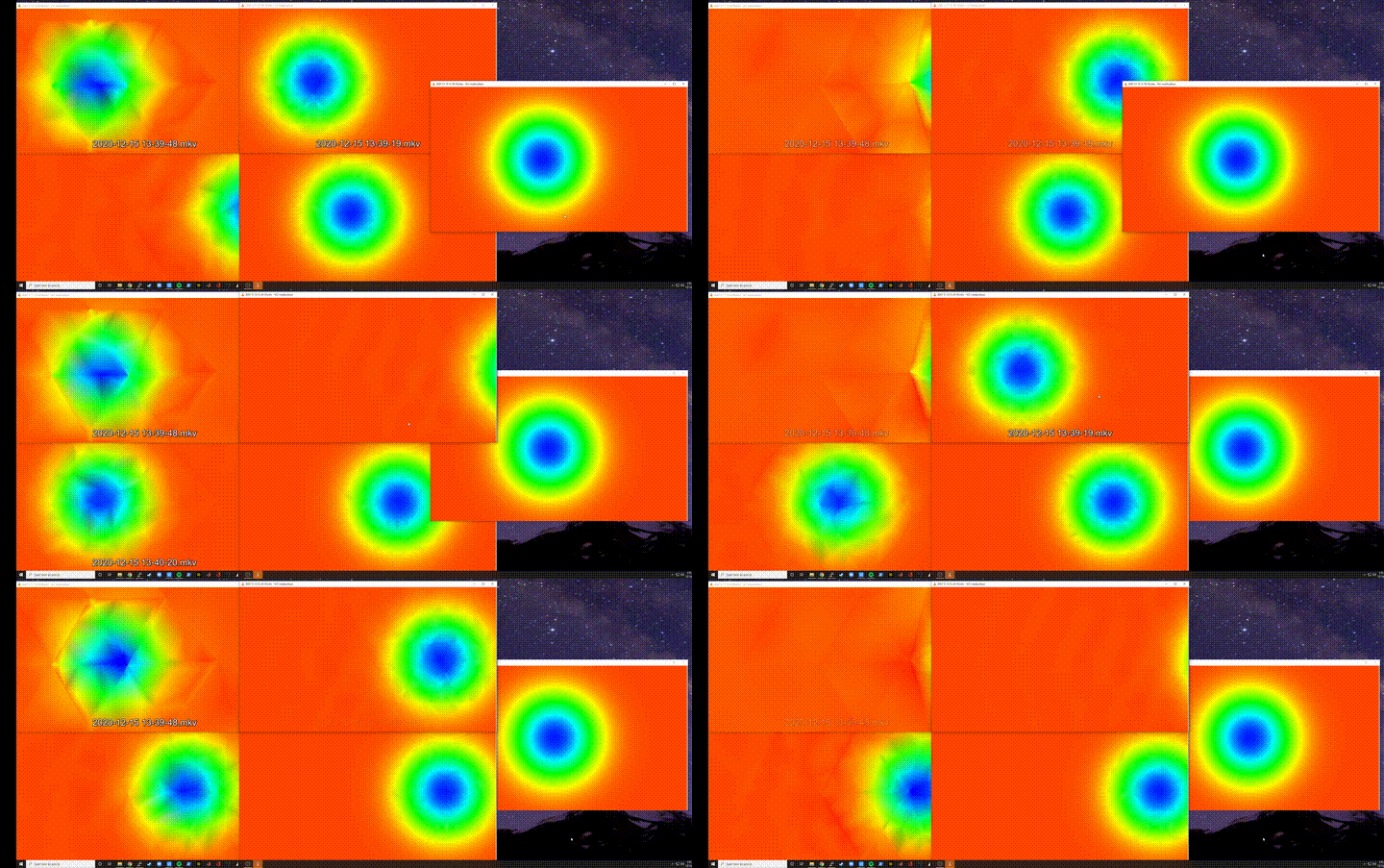
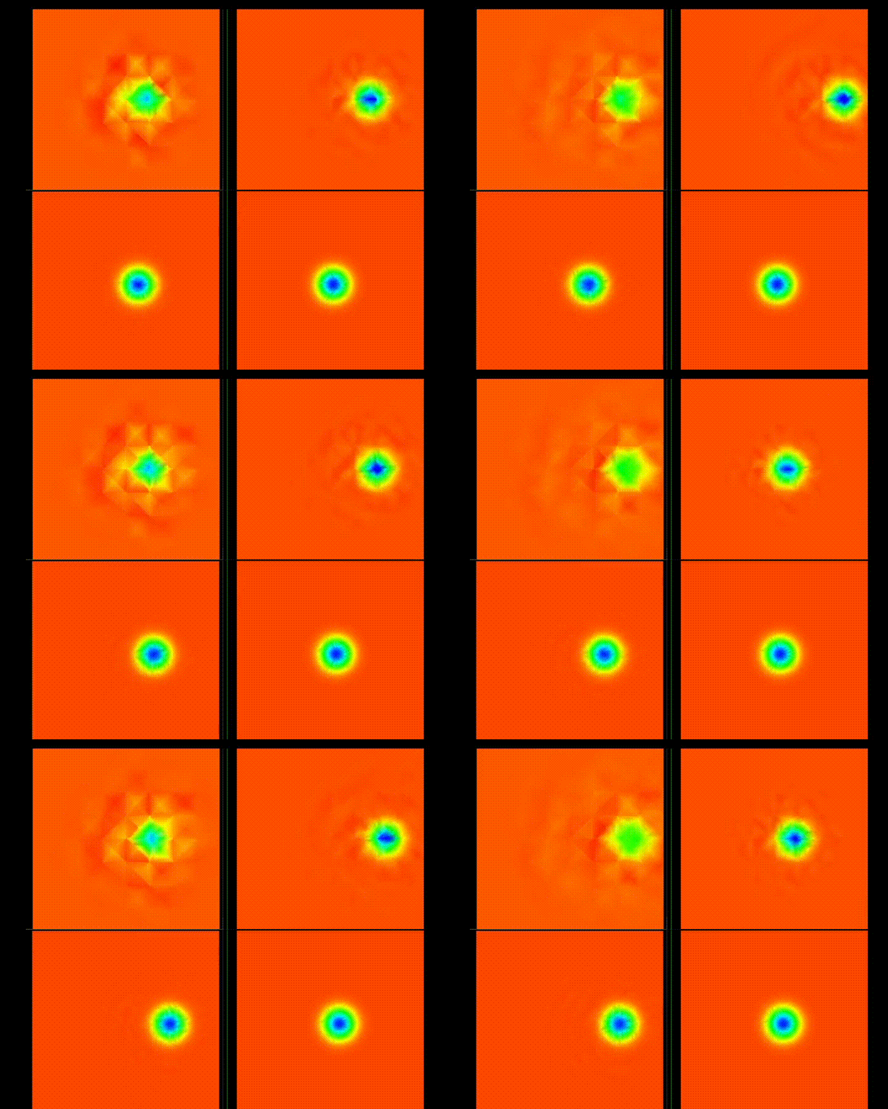
The animation shows a closeup of the isentropic vortex core on three meshes:
- Coarse: 460 triangles
- Middle: 2402 triangles
- Fine: 32174 triangles
On the left is the coarse mesh at Order=2 and Order=4, middle is the same for the medium mesh and on the right is the fine mesh at Order=2. We can see the benefits of both h (grid density) and p (polynomial degree) scaling and we can also see the time penalty for each increase in h or p density.
This current work includes the use of periodic boundary conditions for the right and left boundaries, which works really well.
Next up: solid wall BCs so we can run airfoils, cylinders, etc etc.
The 2D Euler solver now works! Yay!
I've tested the Isentropic Vortex case successfully using a Lax flux and a Riemann BC backed by an analytic solution at the boundaries. Unlike the DG solver based on integration in Westhaven, et al, this solver is not stable when using a Dirichlet (fixed) BC set directly to the analytic solution, so the Riemann solution suppresses unstable waves at the boundary. I haven't calculated error yet, but it's clear that as we increase the solver order, the solution gets much more resolved with lower undershoots, so it appears as though a convergence study will show super convergence, as expected.
The solver is stable with CFL = 1 using the RK3 SSP time advancement scheme. I'll plan to do a formal stability analysis later, but all looks good! The movie below is 1st Order (top left), 2nd Order (top right), 4th Order (btm left) and 7th Order (btm right) solutions of the isentropic vortex case with the same 256 element mesh using a Lax flux. We can see the resolution and dispersion improve as the order increases.
You can recreate the above with gocfd 2D -g --gridFile DG2D/vortexA04.neu -n 1, change the order with the "-n" option. "gocfd help 2D" for all options.
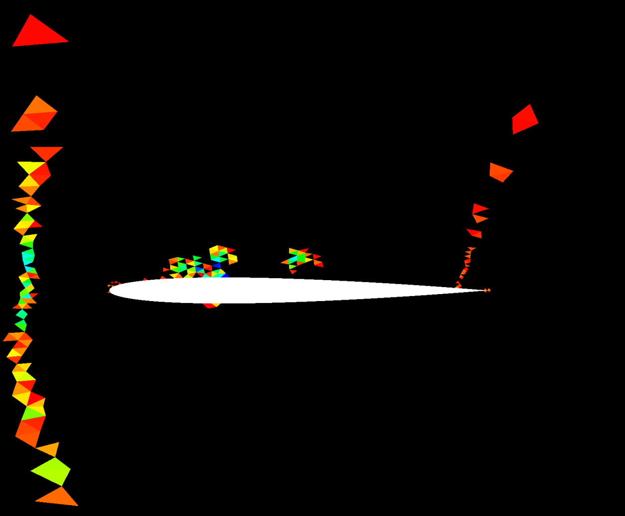
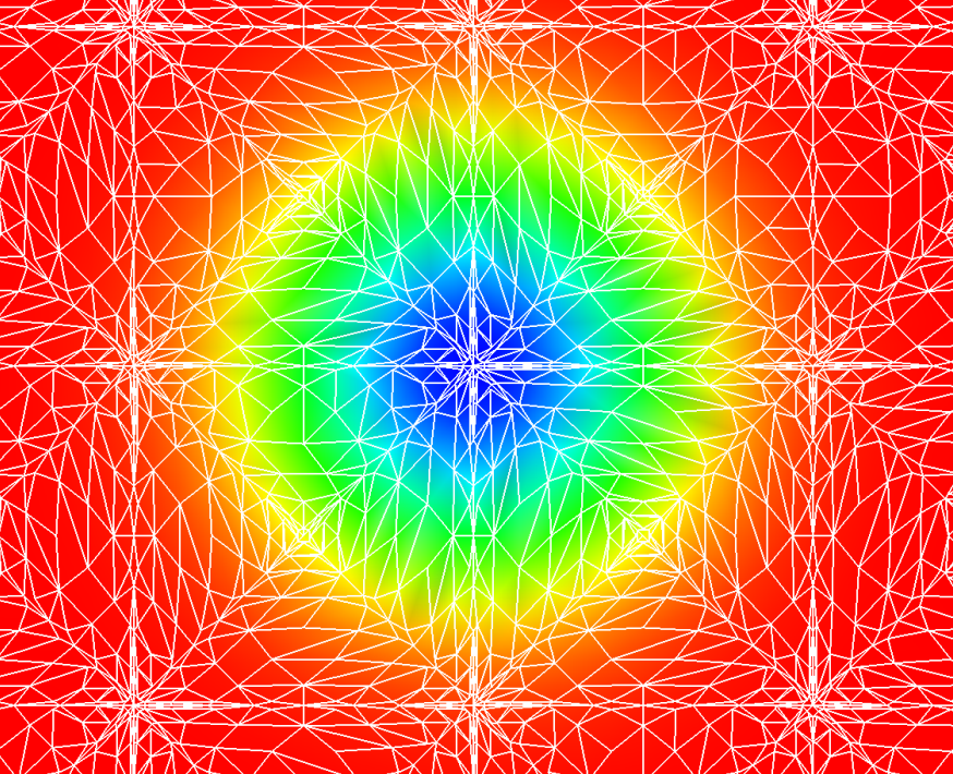
Graphics :-D Very happy to see the first avs renderings of the 2D density! This is a 7-th order mesh, zoomed in on the center of the initial solution for the isentropic vortex.
For comparison - here is a first order version of the same view. You can see the triangulation detail - note that there is a nested triangle configuration, a larger layer of triangles has within it a set of internal triangles. Those are the nodes of the finite elements, and the triangulation inside the larger triangles is a Delaunay triangulation, intended to be used as a linear approximation to the polynomial field.
The 2D Euler solver is functionally complete now, although lacking (many) boundary conditions, the Roe and Lax flux calculations and testing / validation. I want to display the solution graphically to debug.
Next up: graphics to display the solution on the full set of polynomial nodes. Graphics will be key to debugging and answering questions like: "is it better to interpolate flux or solution values, then compute flux?" My plan is to export the triangulation of the RT or Lagrange elements to the graphics plotting in AVS. One question to address: how to handle the corners of the triangles? Currently, the corners are not present in the RT or Lagrange elements - we only have edges up to the corner and interior points. I think that I would rather average the two closest edge points to create the corner value than interpolate corners - my rationale is that I don't want to create artificial extrema in the solution while plotting, it can distract from the actual, and likely problematic extrema I'm seeking to plot.
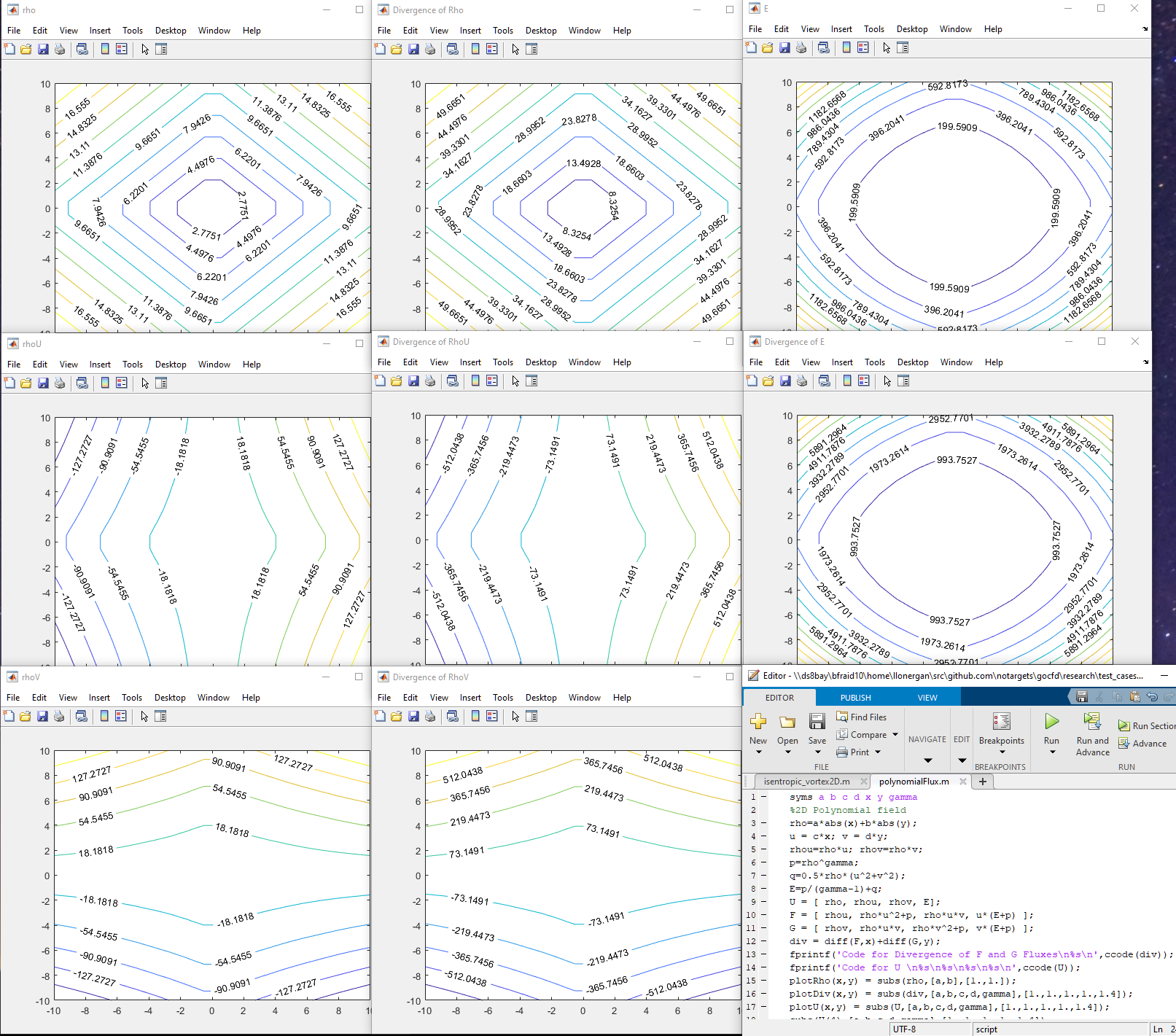
Testing the calculation of divergence using an exact polynomial flux field calculated in Matlab. It seems there's a bug involving the indexing or process using the full transformed calculation with edge computations because the divergence is nearly exact for the first element (k=0) and the mass equation divergence, but deviates for other elements and equations. It's very useful at this point to verify the accuracy of the divergence operator because the bulk of the solver relies on this one operator, and so we can characterize the accuracy (and stability) of the algorithm almost entirely by evaluating the divergence.
Above we see the polynomial flux field in a series of graphs for each equation in the conservative variables and the resulting divergence for each equation. All values are real, not complex and appear smooth (and thus differentiable!).
Progress on the 2D Euler equations solution! There are now unit tests showing that we get zero divergence for the freestream initialized solution on a test mesh. This includes the shared face normals and boundaries along with the solution interpolation. The remaining work to complete the solver includes boundary conditions and the Roe/Lax Riemann flux calculation at shared faces - each of which are pure local calculations.
I'm very happy with the simplicity of the resulting algorithm. There are two matrix multiplications (across all elements), a matrix multiplication for the edge interpolation and a single calculation per edge for the Riemann fluxes. I think the code is easily understood and it should be simple to implement in GPU and other parallel systems.
Divergence is now tested correct for transformed triangles, including the use of the ||n|| scale factor to carry ((Flux) dot (face normal)) correctly into the RT element degree of freedom for edges.
I'm working now on the actual data structures that will efficiently compute the flux values, etc., with an eye on the memory / CPU/GPU performance tradeoffs. Contiguous space matrix multiplications are supported well by GPU, so I'm focusing on making most everything a contiguous space matrix multiply.
Up next: I'm working on initializing the 2D DFR solution method. My plan is to construct a separate structure containing all faces such that we can iterate through the face structure to construct the fluxes on each face only once. Each face is shared by two elements, and each face has a complex and expensive flux construction that unifies the computed values from each element into a single flux shared by both. By constructing a dedicated group of faces, we can iterate through them in parallel to do that construction without duplication. The shared flux values will be placed directly into the flux storage locations (part of the RT element) so that the divergence can be calculated to advance the solution.
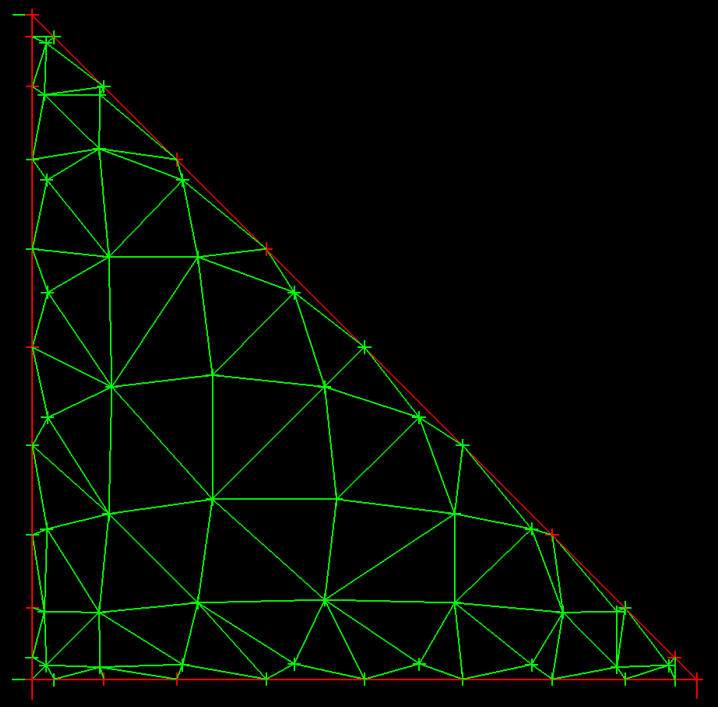
Above we see three elements and within each are the interior solution points and along the edges/faces are the flux points for Order = 1. Each RT element has 12 points, 3 on each face and three interior, while the three Order 1 solution points are in the interior.I've implemented a Delaunay triangulation that converts 2D point fields with fixed boundaries into a triangle mesh. The picture shows the RT7 element triangulated using the method. Now we can use the triangulation within the reference element to implement contour tracing and other graphics to display the field contents within the high order elements. This approach requires that we triangulate only the reference element, then we use that triangulation to fill the insides of the triangles in the mesh (using the affine transform).
I'm adding a contour plotting capability that will provide display of functions within the model. The approach I'm favoring is to triangulate the points within the full RT element, including the vertices, which will enable the plotting of the interpolated solution values used for the edge flux definitions in addition to the interior solution points.
The triangulated mesh containing vertices, the interior solution points and the edge flux points is then used for a linear contour algorithm to produce the isolines for the whole mesh. The resulting isoline field is a linearized view of the polynomials, but is sampled at the full resolution of the polynomial basis at N+1, which should provide an accurate representation of the solution field, though not at the same polynomial order. This should be very useful for visually characterizing the interpolation to the flux points on edges and other attributes of the solution process, in addition to showing actual solutions with high fidelity.
I've now validated the RT element up to 7th order for divergence of polynomial vector fields. Happily, the special case of zero divergence is being captured with high precision.
The reason this took me quite a while: the choice of basis functions for the RT polynomial must be approached with great care, as the derivatives of the basis must be normalized properly. The literature provides many examples of alternatives for the basis, many of which seem to produce erroneous divergence values that do not show convergence, or even diverge with increasing element order. Others use moments of dot products for the interior, which is not the same process that is used by Jameson and Romero's DFR work. In the interest of staying close to that work, I ended up using the same 2D polynomial basis for the Simplex (triangle) as used by Westhaven with the procedure described by Romero to create the basis for the RT element, which preserves the connection with the Lagrange element interior points. I now have validated that this combination accurately reproduces divergence for polynomial functions and shows convergent behavior with good accuracy for transcendental fields up to 7th order.
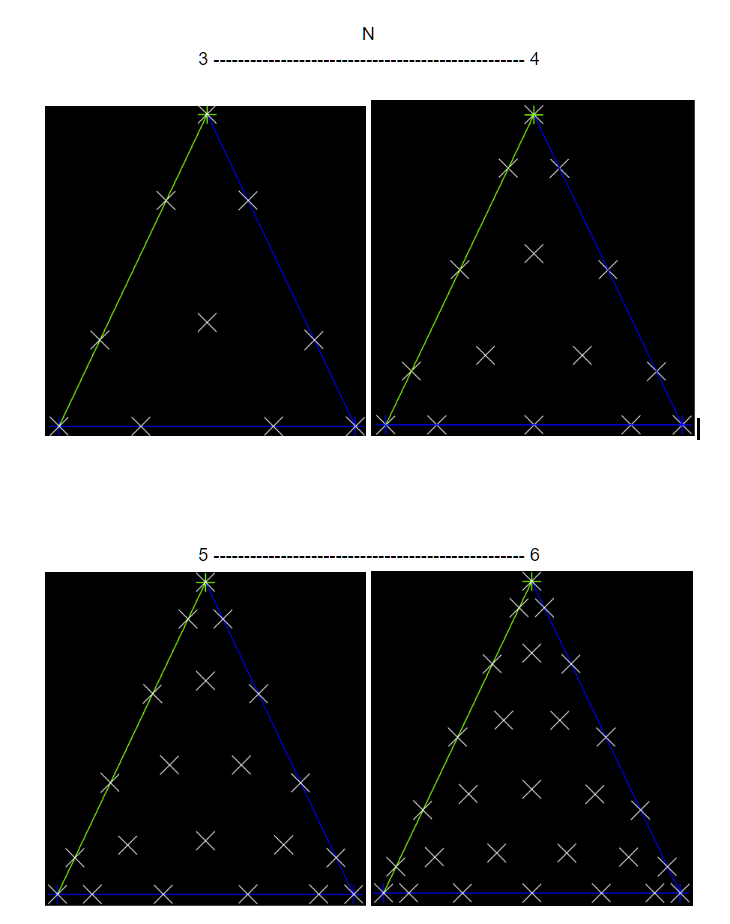
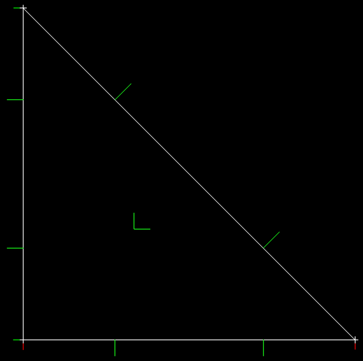
I finally have a working Raviart-Thomas element at any K up to 7th order now. The limitation to 7th order is a matter of finding optimized point distributions for this element type. This RT element closely follows the approach described in Romero and Jameson for the 3rd and 4th orders, and uses the point distributions from Williams and Shun for orders 1,2 and 5-7. The RT vector basis cooefficients for order N are solved numerically in one matrix inversion, yielding a full polynomial basis with (N+1)(N+3) terms implemented as degrees of freedom defining the basis distributed on the [-1,-1] reference triangle. There are 3(N+1) points on the faces of the triangle, and N(N+1)/2 points defining the interior, and each of the interior points hosts 2 degrees of freedom, one for each orthogonal basis vector [r,s] = [1,0] and [0,1], the axis vectos for r and s. The zero order (N=0) element has 0 interior points and 3 face points, one on each face, the N=1 element has 2 points on each face and 1 point in the interior, the N=2 has 9 points on faces (3 per edge), and 3 interior points, for a total of (2+1)(2+3)=15 degrees of freedom.
| RT0 Element | RT7 Element |
|---|---|
 |
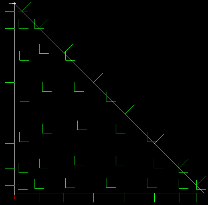 |
The Raviart-Thomas elements at orders 1 and 7 are shown above, with basis vectors as green lines. On the left is RT1, showing a single interior point with two basis vectors. The RT7 element has 28 interior points, each with two basis vectors. The edges of RT7 each have 8 points, each with a single normal vector for the basis.
Here is the cool part: the number of interior points within each of the above elements matches that of the Lagrange element used for the Nodal Galerkin models(!) That means we can have a Nodal Galerkin element at order N=1, which has (N+1)(N+2)/2 = 3 points inside it have a companion RT_2 element that also has 3 interior points. This makes it possible to represent gradient, curl, and divergence of our scalar variables residing inside the Nodal Galerkin elements in the RT_N+1 elements, where those fields are calculated using the two dimensional polynomial basis in a vector preserving way. All this without interpolating between the Lagrangian element and the RT element - the point locations are shared between them, which removes a major source of error and complication.
I'm still implementing tests, but the basics are finally there. Next step: implement gradient, divergence, curl operators and test for convergence to known solutions to [ sin(y), sin(x) ]. After that, I'll need to implement the calculation of the coordinate transform Jacobian, which actually follows from the previous operators in that the calculation of [ J ] includes the same derivatives used in the gradient.
Researching the use of the Raviart-Thomas finite element to represent the numerical flux and divergence.
I've found a lot of good material on these elements and the Raviart-Thomas element, but I'm struggling to find a simple connection between the convenient techniques used for Lagrange elements as expressed in the Hesthaven text and non-Lagrangian elements. In particular, the Lagrange elements have the property that the interpolation operator and the modal representation are connected simply through the Vandermonde matrix. This enables the easy transformation between function values at nodes within the element and interpolations and derivatives. If we could use a Raviart-Thomas element similarly to a Lagrange element, we'd just compose a Vandermonde matrix and proceed as normal to compute the divergence, but, alas, I've struggled to find a way to do this.
I have found the open source element library "Fiat", part of FEniCS, that implements RT elements and will produce a Vandermonde matrix for them, but I'm not convinced it's useful in a way similar to Lagrange elements. Also, I found that the ordering of the polynomial expansions are strange in the RT elements in Fiat - not sure it matters, but it's not a straightforward "smallest to largest" ordering, which brings into question how to use that Vandermonde matrix in general.
So - I'm back to basic research on the meaning of finite elements and how to properly represent the flux on Raviart-Thomas elements. Papers I'm reading can be found here.
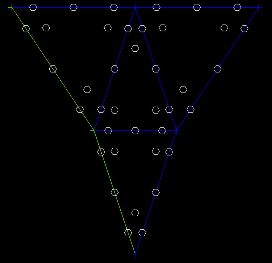
Experimenting with node distributions - shown are the LGL points with warping per the Hesthaven approach.
Unsolved/undecided: Is it a good idea to use the next higher order LGL points for the flux and interpolate down to the solution points from there? This question arises because, unlike in the 1D case, there isn't an overlapping points group like the Gauss points for the interior and the LGL points at one higher polynomial degree, which conveniently accomplished having colocated solution and flux points in the interior. Instead, as can be seen in the above graphic - the interior points are at very different locations between orders (eg N=3 compared with N=4), so every transfer from flux points and solutions points will involve interpolation between points. This introduces interpolation errors I'd like to avoid...
Given that for a given multidimensional polynomial degree N the number of polynomial points needed is (N+1)(N+2)/2, so it seems impossible to find a distribution of points that would overlap as in the 1D case.
Implemented a Gambit formatted mesh reader and updated AVS to plot tri meshes.
Success!
I reworked the DFR solver and now have verified optimal (N+1) convergence on the Euler equations for a density wave (smooth solution). The convergence orders for N=2 through N=6 are:
DFR Integration, Lax Friedrichs Flux
Order = 2, convergence order = 2.971
Order = 3, convergence order = 3.326
Order = 4, convergence order = 4.906
Order = 5, convergence order = 5.692
#Affected by machine zero
Order = 6, convergence order = 3.994

DFR Integration, Roe Flux
Order = 2, convergence order = 2.900
Order = 3, convergence order = 3.342
Order = 4, convergence order = 4.888
Order = 5, convergence order = 5.657
#Affected by machine zero
Order = 6, convergence order = 4.003
Note that:
- No limiter is used on the smooth solution
- Odd orders converge at something less than the optimal rate
- Even orders converge at approximately N+1 as reported elsewhere
I've noticed dispersion errors in the odd order solutions for the SOD shock tube when using a limiter - the shock speed is wrong. I'm not sure what causes the odd orders to behave so differently at this point. The difference in convergence rate between even and odd orders suggests there may be a material issue/phenomenon for odd orders, though I haven't found anything different (like a bug) in the process, which leads to a question about the algorithm and odd orders. One thing to think about: Even orders put a solution point in the center of each element, while odd orders do not...
At this point I feel confident that I'm able to move on to multiple dimensions with this approach. I'll definitely need to implement a different and/or augmented limiter approach for solutions with discontinuities, likely to involve a "shock finder" approach that only uses the limiter in regions that need it for stability.
A note on the refactored DFR approach: In the refactored DFR, an N+2 basis is used for the flux that uses (N+3) Legendre-Gauss-Lobato (LGL) points, which include the edges of each element. The solution points use a Gauss basis for the element, which does not include the edge points, and there are (N+1) interior points for the solution. At each solver step, the edge points of the solution are interpolated from the (N+1) solution points to the edges of the (N+3) flux basis and then the flux is computed from the solution primitive variables. The derivative of the flux is then computed on the (N+3) points to form the solution RHS components used in the (N+1) solution. The result is that the flux is a polynomial of order (N), and so is the solution.
Below is:
Euler Equations in 1 Dimension
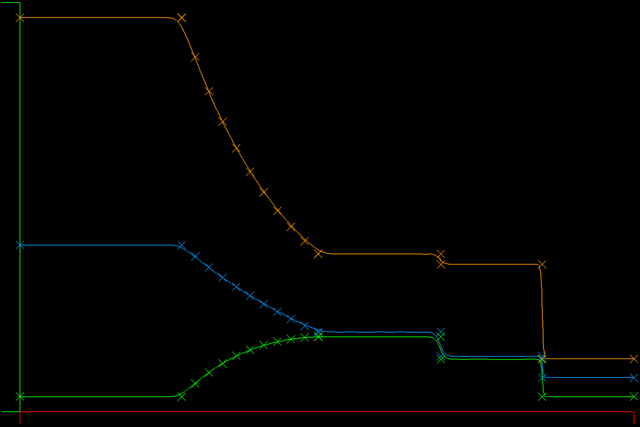
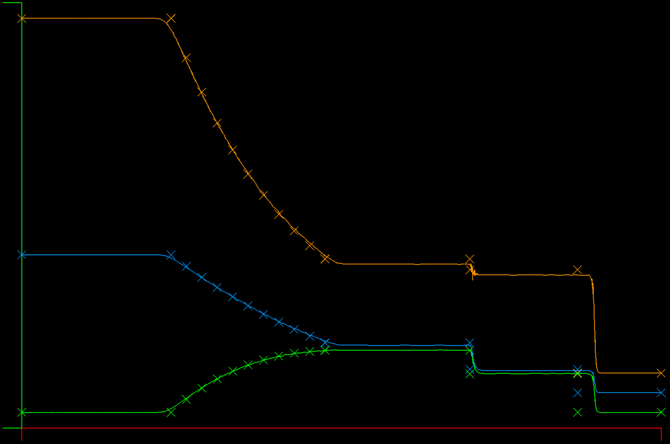
Solving Sod's Shock Tube
Algorithm: DFR Integration, Roe Flux
Solution is limited using SlopeLimit
CFL =   2.5000, Polynomial Degree N = 8 (1 is linear), Num Elements K = 2000

SOD Shock Location = 0.6753
Rho Integration Check: Exact = 0.5625, Model = 0.5625, Log10 Error = -4.3576
case,K,N,CFL,Log10_Rho_rms,Log10_Rhou_rms,Log10_e_rms,Log10_rho_max,Log10_rhou_max,Log10_e_max
"DFR Integration, Roe Flux",2000,8,2.5000,-2.6913,-2.7635,-2.2407,-1.7183,-1.6491,-1.1754
Implemented a smooth solution (Density Wave) in the Euler Equations DFR solver and ran convergence studies. The results show a couple of things:
- Rapid convergence to machine zero across polynomial order and number of elements
- Order of convergence is N, not the optimal (N+1)
- Aliasing instability when using the Roe flux
- The "SlopeMod" limiter destroys the accuracy of the smooth solution
While it was very nice to see (1) happen, the results of (2) made me take a harder look at the DFR approach implemented now. I had taken the "shortcut" of having set the flux at the element faces, and not modifying the interior flux values, which has the impact of converting the flux into a polynomial of order (N-2) due to the removal of the two faces from the order N basis by forcing their values. It seems that the resulting algorithm has a demonstrated order of (N-1) in convergence rate as a result.
One of the reasons I took the above shortcut is that right now we are using the "Legendre-Gauss-Lobato" (LGL) nodes for the algorithm, per Hesthaven, and the LGL points include the face vertices for each element, which makes it impossible to implement the Jameson DFR approach for DFR.
In the Jameson DFR, the Gauss quadrature points do not include the face vertices. The algorithm sets the flux values at the face vertices, then performs an interpolation across the combination of interior and face (N+1+2) vertices to determine the coefficients of the interior flux polynomial such that the new polynomial passes through all (N+1) interior points in the element and the two face vertices. The resulting reconstructed flux polynomial is of order (N+2) and resides on the (N+3) face and solution interior points. Derivatives of this flux are then used directly in the solution algorithm as described in this excellent AFOSR presentation.
The Jameson DFR algorithm provides an equivalent, but simpler and more efficient (15% faster) way to achieve all of the benefits of DG methods. The DFR solver uses the differential form of the target equations, rather than the integral form, which makes it easier to attack more complex combinations of target equations. DFR has also been extended by Jameson, et al to incorporate spectral methods with entropy stable properties.
Updates (May 26, 2020): Verified DFR and Roe Flux after fixing the Exact solution to the Sod shock tube
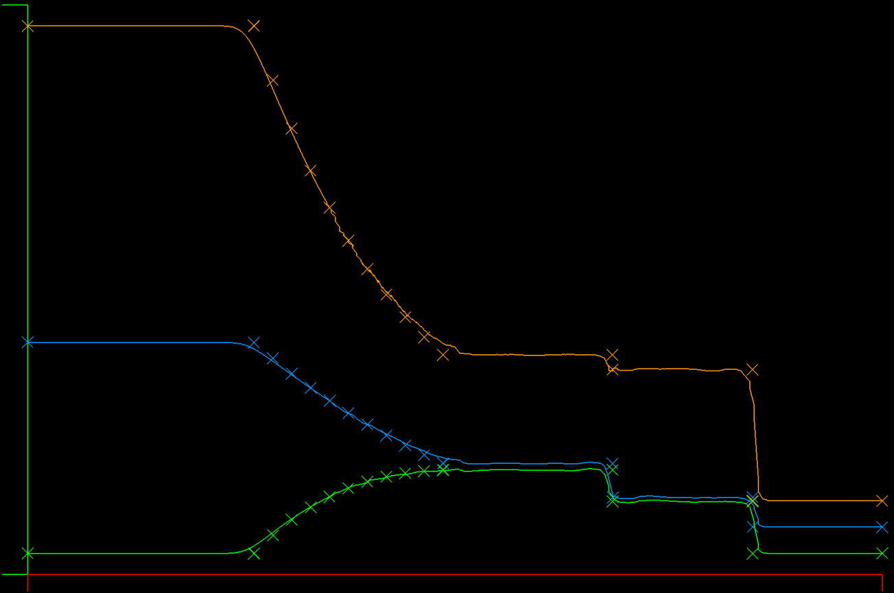
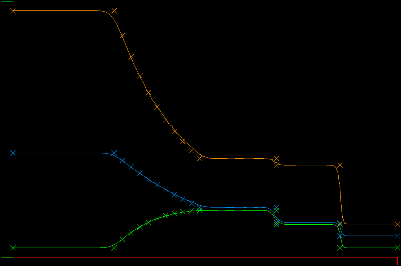
A highly resolved solution from the DFR/Roe solver looks qualitatively good without bumps or other instability artifacts. The contact discontinuity is in the right place and very sharply resolved.
| DFR Roe (fixed flux) | Galerkin Lax |
|---|---|
 |
 |
I removed a term that was present in the 3D version of the flux that doesn't make sense in 1D, and now the contact discontinuity is in the right place and the bump is gone.
Now, when we compare the DFR Roe flux (left) to the Galerkin Lax flux (right), we can see the Roe solution has a steeper contact discontinuity and shock, as we would expect. Both solutions get the locations correctly.
I also optimized some of the DFR code and timed each solution. Surprisingly, the DFR/Roe is slightly faster than the Galerkin/Lax.
| DFR Roe (broken flux) | Galerkin Lax |
|---|---|
 |
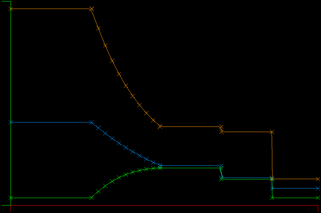 |
DFR/Roe versus Galerkin/Lax: In the DFR solution the contact discontinuity is steeper than the GK/Lax solution. There is a very slight position error for the contact discontinuity in the DFR solution and also a bump on the left side of it, an artifact of the underdamped aliasing.
The shock speed problem I saw yesterday turns out to have been the exact solution :-)
After correcting the exact solution to Sod's shock tube problem, the two Euler solvers match up pretty well all around, with some small differences between them - phew!
This is cool - being able to see exactly the errors and successes in realtime. The above is a snap of an interim result where I'm now showing the exact solution in symbols overlaying the simulation in realtime and sure enough we see a shock speed error on the leading shock wave, along with excellent reproduction of the smooth expansion flow.
I also went back and checked the Galerkin (non-DFR) Euler case and it has the same error in shock propagation speed as the DFR/Roe result, which says there's a common error somewhere. It's good to spend time doing basic accuracy tests!
You can recreate this using gocfd -graph -model 5 -CFL 0.75 -N 4 -K 600
On the path to implementing direct flux reconstruction, I found what appeared to be 2nd order aliasing without a clear origin. After consulting Hesthaven(2007) section 5.3, I see that the issue is the interpolation of the flux and subsequently taking the derivative of that interpolated flux. As stated: "the derivative of the interpolation is not the same as the interpolation of the derivative", or put another way, by simply computing the flux from the nodal points of the solution polynomial, we are not treating the flux formally as a polynomial - instead we should perform a formal polynomial fit (projection, instead of interpolation) of the flux prior to using that polynomial to compute derivatives of the flux. The result of using interpolation shown in the text is that we produce an aliasing error into the solution, and their answer is to filter it away instead of using the much more compute intensive projection. The aliasing error also gets worse with increasing N, so the filter should change with N.
I've implemented a simple 2nd order dissipative filter with a constant coefficient, which works well to knock out the oscillations without introducing solution error. I also experimented with a combined 2nd / 4th order filter, similar to what is commonly used in finite volume schemes and for this problem the 2nd order dissipation was enough. However, I can not get stable results beyond about N=6 with this filter, so I'll also investigate an efficient way to do projection and/or improved filters.
--> prior updates DFR for Maxwell's equations now uses 2nd order artificial dissipation to remove the odd/even aliasing and it works pretty well, which affirms my earlier finding of higher order modes. Next steps might include doing a stability analysis on the DFR scheme, covering the details of the reconstruction. It is slightly different than in Jameson(2014), in that this formulation of NDG uses N+1 points for the polynomials, including the node edges. In Jameson(2014), they extended the flux points to N+3 to cover the element edges, where here I just formed the fluxes at the face points, which are at i=1 and i=N+1.
You can see it as model 4 with default parameters like gocfd -model 4 -graph The issue is the instability - it scales with N, so is a higher order modal signal - It could be that the Lax Friedrich's flux, which is 1st order, is not providing damping of the higher order modes. But why are there higher order modes? Are these unresolved waves? I can't answer without more looking into it...
Current Status (May 9, 2020): Direct Flux Reconstruction implemented for 1D Advection, moving to implement for the other two 1D model problems
DFR works for Advection (-model 3) and seems to improve accuracy and physicality.
The primary differences between using DFR and traditional Nodal Discontinuous Galerkin:
- Instead of using only the primitive variables in the right hand side, we use the Flux directly for a hyperbolic problem
- The flux is a globally composed variable and is differentiated after being "reconstructed" to be C(0)
- The reconstruction technique follows Jameson(2014) in that we coerce the flux values of each face to be consistent values at each face, then use the same Np Gauss-Lobato nodes and metrics to develop the derivative(s) of flux
For (3) in this case, I used the same Lax-Friedrichs flux calculation from the text, then averaged the values from each side of each face together to make a single consistent face value shared by neighboring elements.
During testing of the method in 1D as outlined in the text, it became clear that the slope limiter is quite crude and is degrading the physicality of the solution. The authors were clear that this is just for example use, and now I'm convinced of it!
My first round of research yielded the Direct Flux Reconstruction technique from a 2014 paper by Antony Jameson, et al (one of my favorite CFD people of all time). The technique is extremely simple and has the great promise of extending the degree of accuracy to the Flux terms of more complex equations, in addition to enabling the use of flux limiters that have been proven for flows with discontinuities.
In my past CFD experience, discontinuities in solving the Navier Stokes equations are not limited to shock waves. Rather, we find shear flows have discontinuities that are similar enough to shock waves that shock finding techniques used to guide the application of numerical diffusion can be active at the edge of boundary layers and at other critical regions, which often leads to inaccuracies far from shocks. The text's gradient based limiter would clearly suffer from this kind of problem among others.
Here is what I'm using as a platform:
me@home:bash# go version
go version go1.14 linux/amd64
me@home:bash# cat /etc/os-release
NAME="Ubuntu"
VERSION="18.04.4 LTS (Bionic Beaver)"
...
You also need to install some X11 and OpenGL related packages in Ubuntu, like this:
apt update
apt install libx11-dev libxi-dev libxcursor-dev libxrandr-dev libxinerama-dev mesa-common-dev libgl1-mesa-dev
A proper build should go like this:
me@home:bash# make
go fmt ./...  && go install ./...
run this -> $GOPATH/bin/gocfd
me@home:bash# /gocfd$ gocfd --help
Usage of gocfd:
  -K int
        Number of elements in model (default 60)
  -N int
        polynomial degree (default 8)
  -delay int
        milliseconds of delay for plotting (default 0)
  -graph
        display a graph while computing solution
  -model int
        model to run: 0 = Advect1D, 1 = Maxwell1D (default 1)
During testing of the method in 1D as outlined in the text, it became clear that the slope limiter is quite crude and is degrading the physicality of the solution. The authors were clear that this is just for example use, and now I'm convinced of it!
My first round of research yielded the Direct Flux Reconstruction technique from a 2014 paper by Antony Jameson, et al (one of my favorite CFD people of all time). The technique is extremely simple and has the great promise of extending the degree of accuracy to the Flux terms of more complex equations, in addition to enabling the use of flux limiters that have been proven for flows with discontinuities.
In my past CFD experience, discontinuities in solving the Navier Stokes equations are not limited to shock waves. Rather, we find shear flows have discontinuities that are similar enough to shock waves that shock finding techniques used to guide the application of numerical diffusion can be active at the edge of boundary layers and at other critical regions, which often leads to inaccuracies far from shocks. The text's gradient based limiter would clearly suffer from this kind of problem among others.
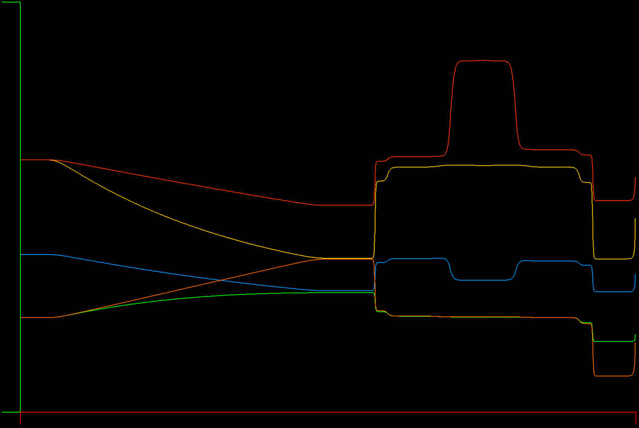
This is an interesting problem because of the temperature remainder after the collision. In the plot, temperature is red, density is blue, and velocity is orange. After the shocks pass out of the domain, the remaining temperature "bubble" can't dissipate, because the Euler equations have no mechanism for temperature diffusion.
This case is obtained by initializing the tube as with the Sod tube, but leaving the exit boundary at the left side values (In == Out). This produces a left running shock wave that meets with the shock moving right.
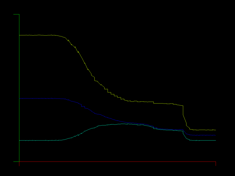
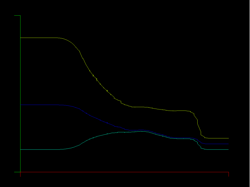
The 1D Euler equations are solved with boundary and initial conditions for the Sod shock tube problem. There is an analytic solution for this case and it is widely used to test shock capturing ability of a solver.
Run the example with graphics like this:
bash# make
bash# gocfd -model 2 -graph -K 250 -N 1
You can also target a final time for the simulation using the "-FinalTime" flag. You will have to use CTRL-C to exit the simulation when it arrives at the target time. This leaves the plot on screen so you can screen cap it.
bash# gocfd -model 2 -graph -K 250 -N 1 -FinalTime 0.2
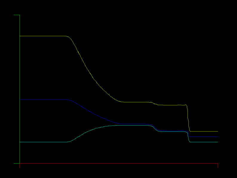
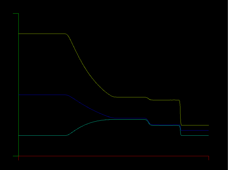
| Linear Elements | 10th Order Elements |
|---|---|
 |
 |
| Linear Elements | 10th Order Elements |
|---|---|
 |
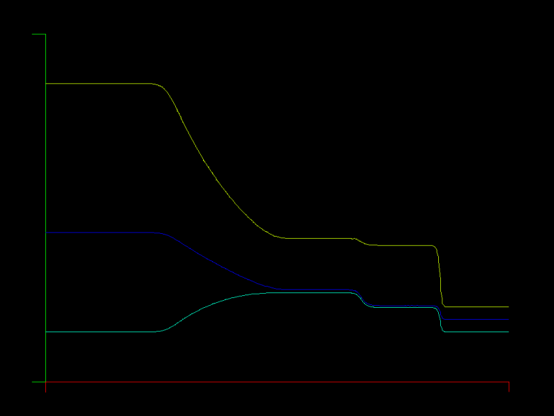 |
| Linear Elements | 10th Order Elements |
|---|---|
 |
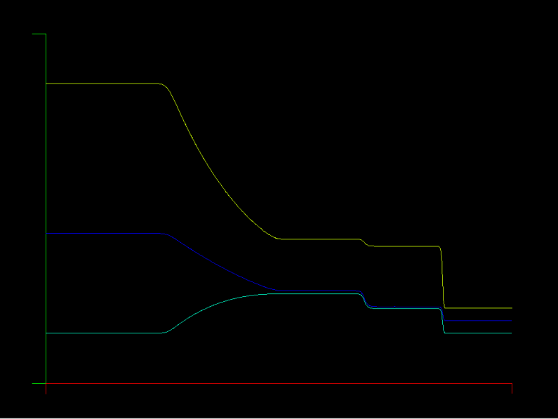 |
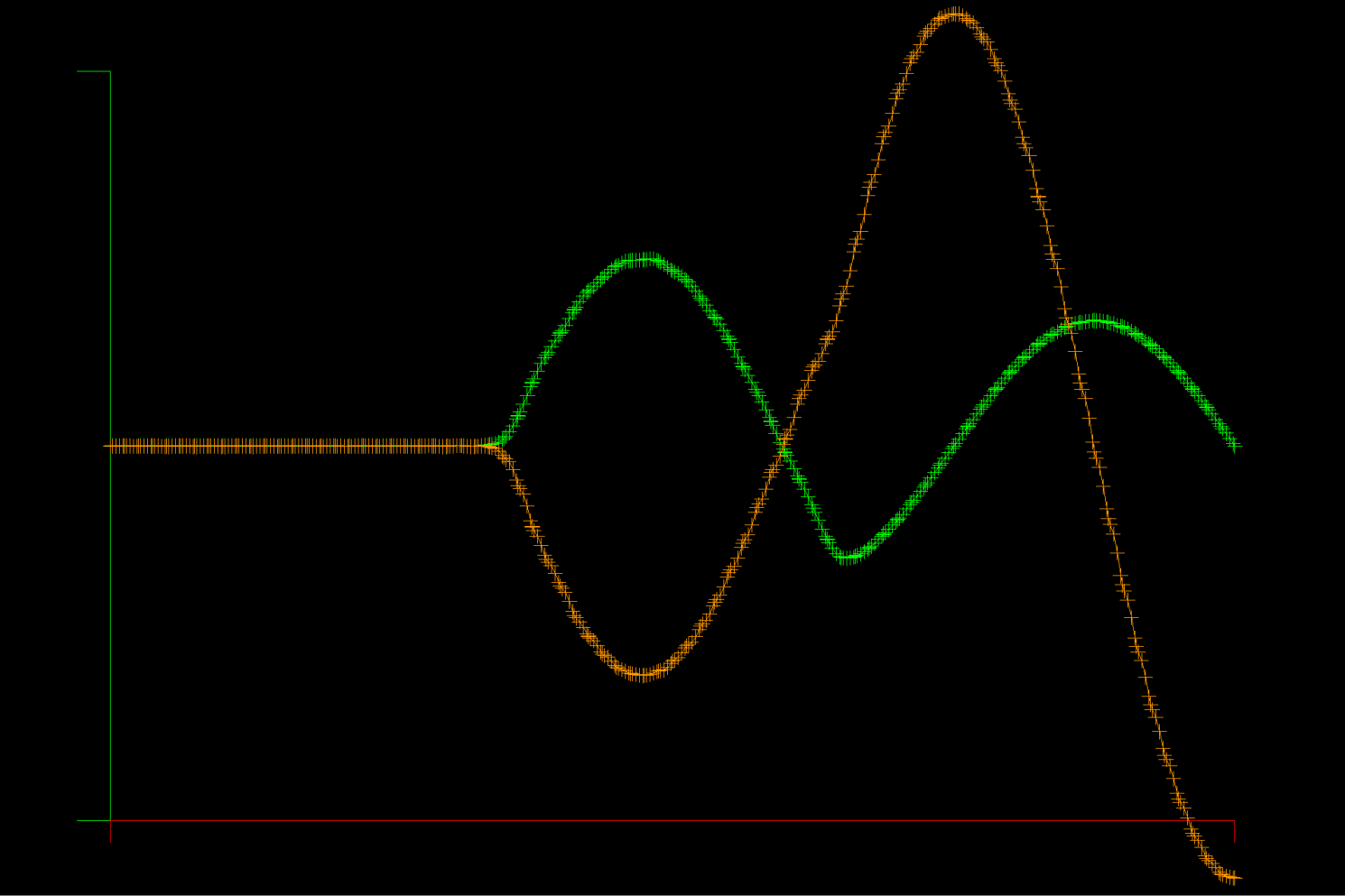
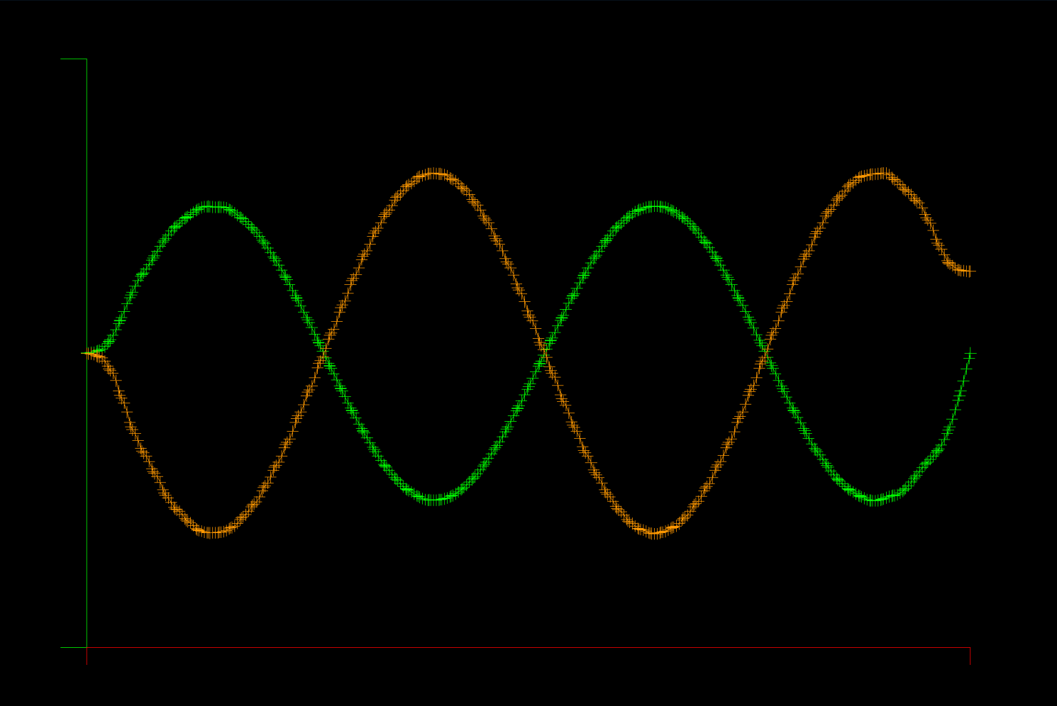
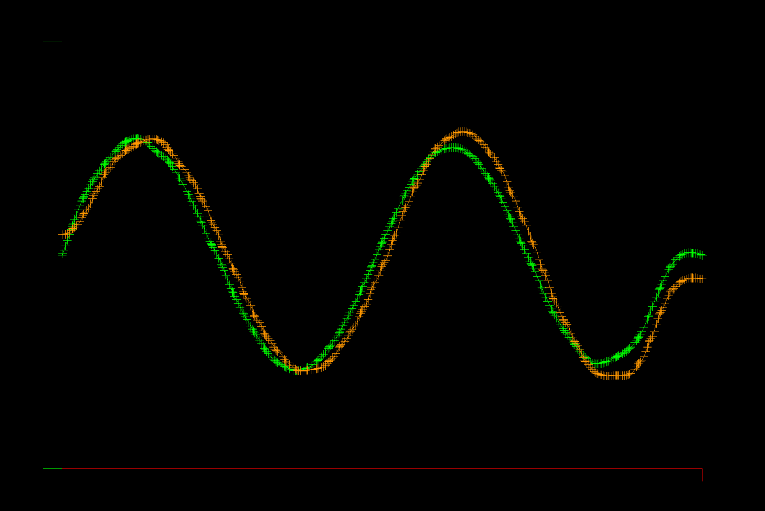
The Maxwell equations are solved in a 1D metal cavity with a change of material half way through the domain. The initial condition is a sine wave for the E (electric) field in the left half of the domain, and zero for E and H everywhere else. The E field is zero on the boundary (face flux out = face flux in) and the H field passes through unchanged (face flux zero), corresponding to a metallic boundary.
Run the example with graphics like this:
bash# make
bash# gocfd -model 1 -delay 0 -graph -K 80 -N 5
Unlike the advection equation model problem, this solver does have unstable points in the space of K (element count) and N (polynomial degree). So far, it appears that the polynomial degree must be >= 5 for stability, otherwise aliasing occurs, where even/odd modes are excited among grid points.
In the example pictured, there are 80 elements (K=80) and the element polynomial degree is 5 (N=5).
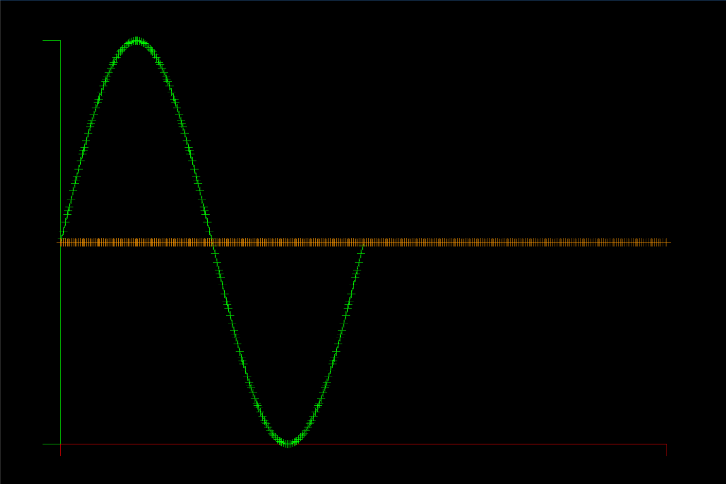
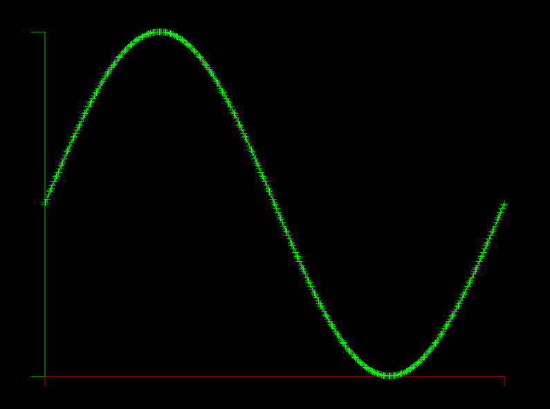
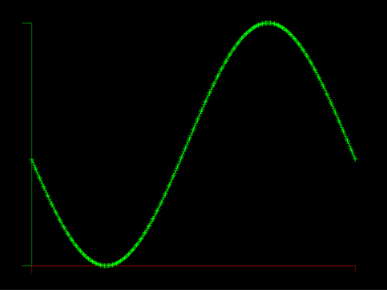
The first model problem is 1D Advection with a left boundary driven sine wave. You can run it with integrated graphics like this:
bash# gocfd -model 0 -delay 0 -graph -K 80 -N 5
In the example pictured, there are 80 elements (K=80) and the element polynomial degree is 5 (N=5).
