The code was developed initially in Python programming language and all computationaly expensive parts are implemented in C++ and CUDA-C++ to allow better optimizations. You can run this software both in a CPU or an NVIDIA GPU. The code is still under development for optimization purpose however it is already fully functional and tested to produce correct results. The code is oriented to run in Linux operating systems, locally or in remote servers.
Python works as the "glue" code that utilizes useful libraries such as numpy, scipy, skimage, unittest etc. that favor development productivity, and at the same time provide sufficient perfromance. For even higher performance we use the module ctypes to interface with C++ or CUDA-C++ compiled code. We suggest to install Python using the Anaconda framework.
To be able to compile the code you need to have installed Intel's Math Kernel Library (MKL) and CUDA, both are available for free download.
- MKL : https://software.intel.com/en-us/mkl/choose-download
- CUDA : https://developer.nvidia.com/cuda-downloads
To run this code you need first to compile the C++ source code which is present in the directory /cpp_src/ using the Makefile in the same directory. To do so, open the Makefile and specify the location of intel mkl directory.
In example:
INTEL = /opt/intel
MKLROOT = $(INTEL)/mkl
When you manage to compile succesfully you should see the following dynamic shared libraries in the same directory.
- extrapolation_cpu.so
- extrapolation_gpu.so
- extrapolation_revOp_gpu.so
The first library provides implementation of extrapolation and imaging on CPU, while the second and third do so for GPU. The third libray is the latest one and generally performs faster. We suggest to use this (in case you want to run on a GPU)!
This code is tested unit-by-unit using the Python module unittest, to ensure correctness. One way to run the code is to run these unit-tests. In the directory /unittests/ you can find all test scripts (test_*.py), as well as three bash scripts to run them. There is one script for the Python codes, one for the C++ and one for the CUDA-C++ codes.
Run as follows:
- bash run-py_src-tests.sh
- bash run-cpp_src-tests.sh
- bash run-cpp_src_cuda-tests.sh
The main Python script (main.py) is found in the top directory. You may run the code using the provided bash script run_demo.sh. Whether you want to run the code on a CPU or GPU you do by specifing your option as command line parameter.
In example, in order to use the CPU implementation (extrapolation_cpu.so), the command is:
- python main.py demo-data/velmod.csv demo-data/problemSetup.txt demo-data/seismicShots/ demo-result host
note the last parameter "host"
In order to use the second library (naive GPU implementation), replace the 5th parameter "host" with "device". To use the third, replace "host" with "device_revOp", like this:
- python main.py demo-data/velmod.csv demo-data/problemSetup.txt demo-data/seismicShots/ demo-result device_revOp
The main Python script (main.py) needs the following 5 command line parameters:
- a comma separated values (CSV) file with the 2D velocity model (see demo-data/velmod.csv)
- a simple txt file with the problem configuration parameters, i.e nz, nx, nf etc. (see demo-data/problemSetup.txt)
- a directory containg (CSV) files where each file contains the signal recorded at the "surface" of the model that you attempt to image. Each file-name must follow the syntax seisX_NX.csv, where X is the position (in x-axis) of the source and NX the range. (see the files in the directory demo-data/seismicShots).
- the output directory (i.e demo-results)
- one of the three options: host, device or device_revOp that indicates where you want the extrapolation and imaging to be computed (CPU, GPU version 1, GPU version 2).
Upon completition the code saves in the specified output directory (parameter 4) the velocity model and accumulated (over all shots) final image as CSV files. You can visualize each with the provided script vis.py.
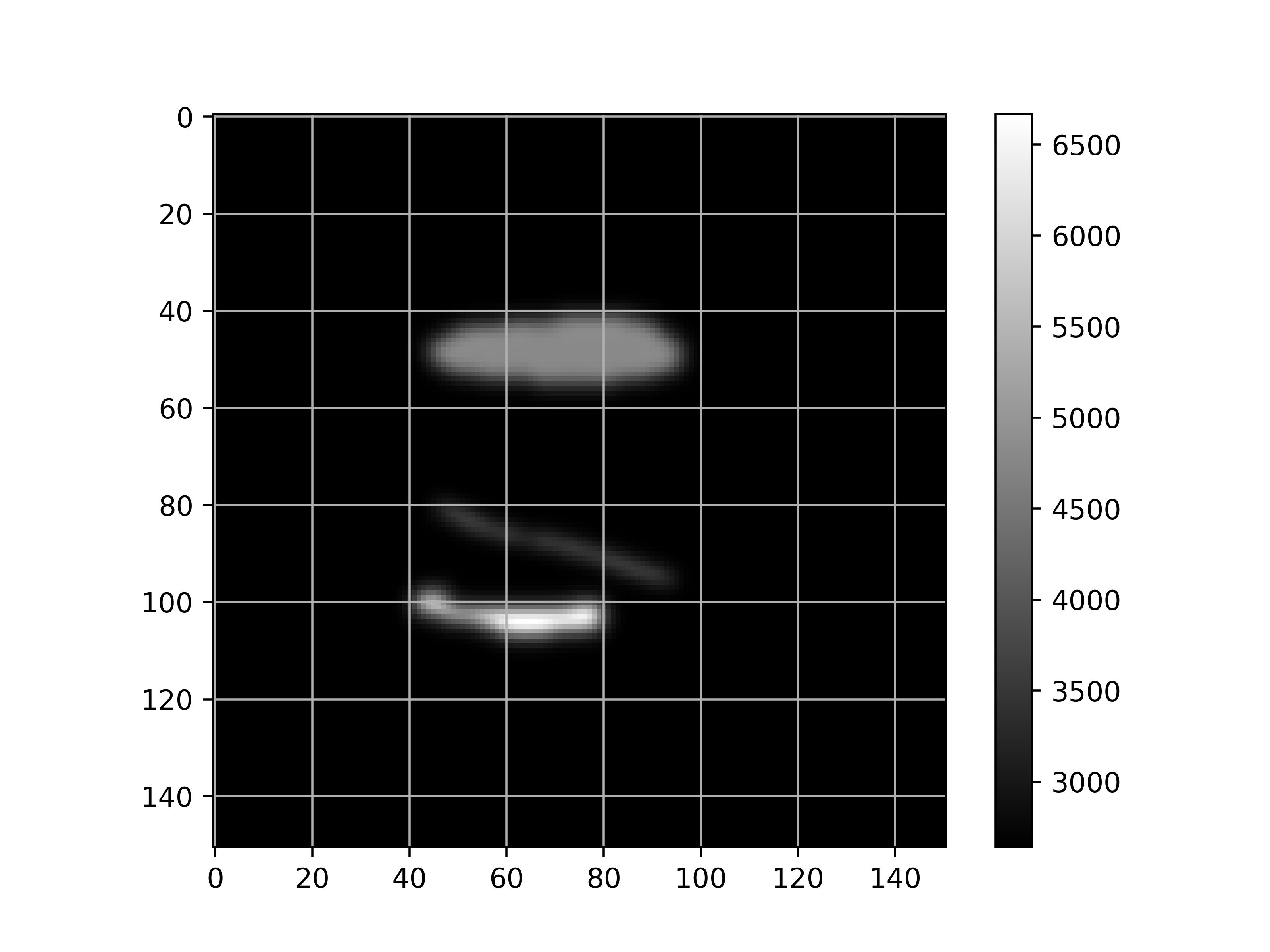
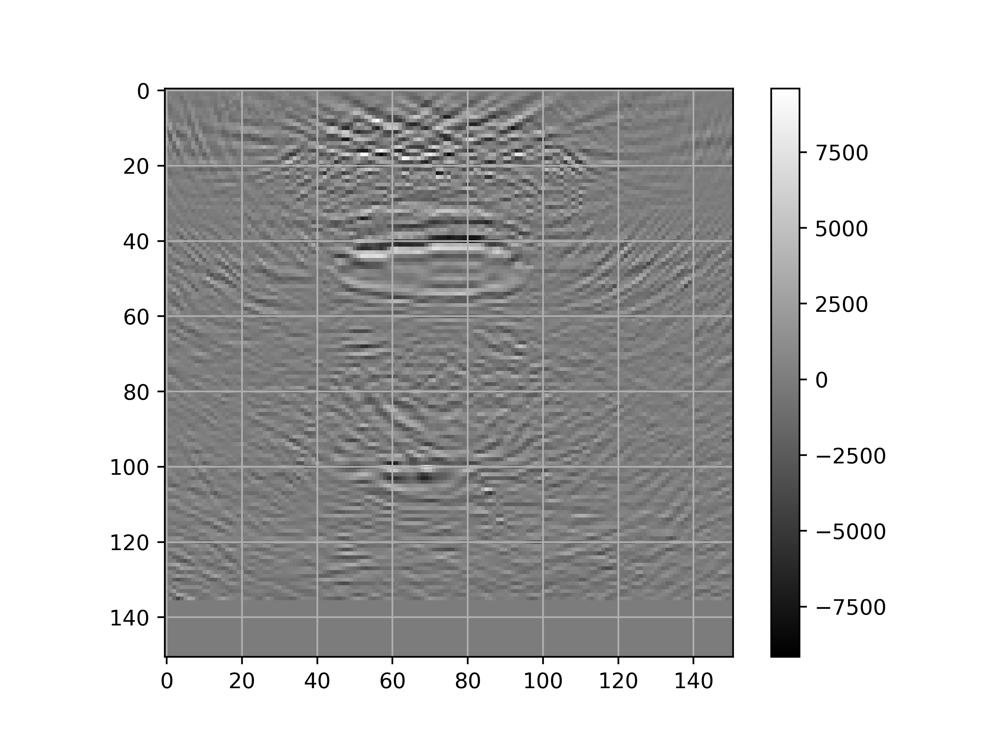
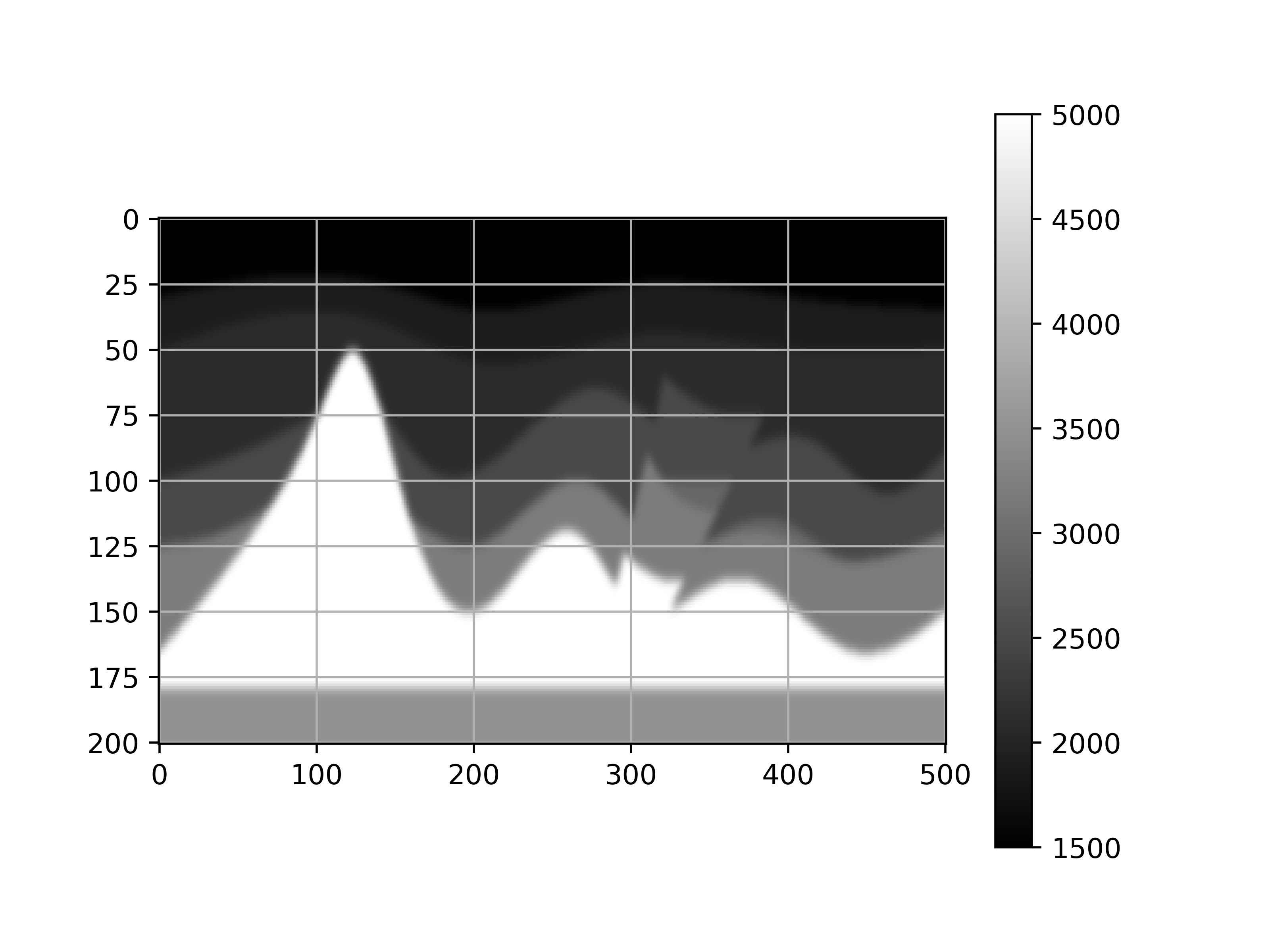
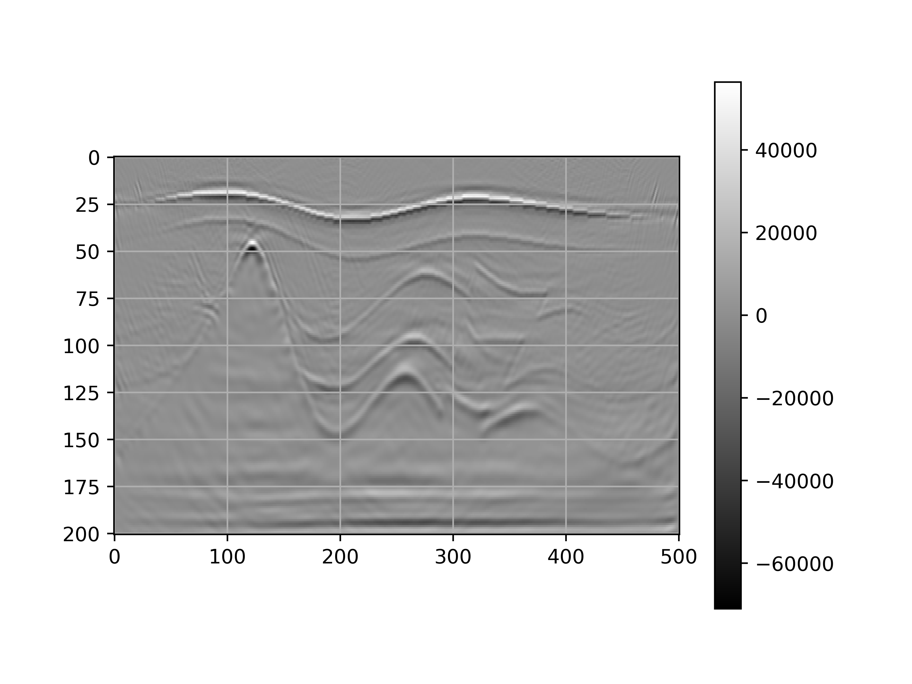
Here are two examples that demonstrate the output of this software. The first (is the provided demo) is an imaging of a poorly sampled experiment and thus there is significant amount of noise in the final image. On the other hand, the two images below correspond to imaging of a denser and more carefully sampled experiment, and therefore leads to a better final image.


