RuCLIP

Zero-shot image classification model for Russian language

RuCLIP (Russian Contrastive Language–Image Pretraining) is a multimodal model for obtaining images and text similarities and rearranging captions and pictures. RuCLIP builds on a large body of work on zero-shot transfer, computer vision, natural language processing and multimodal learning. This repo has the prototypes model of OpenAI CLIP's Russian version following this paper.

Models

Installing

pip install ruclip==0.0.2

Usage

Standart RuCLIP API

RuCLIP + SberVqgan

ONNX example

Init models

import ruclip

device = 'cuda'
clip, processor = ruclip.load('ruclip-vit-base-patch32-384', device=device)

Zero-Shot Classification [Minimal Example]

import torch
import base64
import requests
import matplotlib.pyplot as plt
from PIL import Image
from io import BytesIO

# prepare images
bs4_urls = requests.get('https://raw.githubusercontent.com/ai-forever/ru-dolph/master/pics/pipelines/cats_vs_dogs_bs4.json').json()
images = [Image.open(BytesIO(base64.b64decode(bs4_url))) for bs4_url in bs4_urls]

# prepare classes
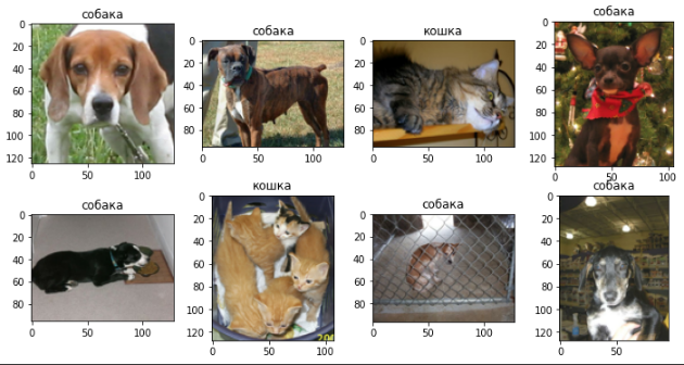
classes = ['кошка', 'собака']
templates = ['{}', 'это {}', 'на картинке {}', 'это {}, домашнее животное']

# predict
predictor = ruclip.Predictor(clip, processor, device, bs=8, templates=templates)
with torch.no_grad():
    text_latents = predictor.get_text_latents(classes)
    pred_labels = predictor.run(images, text_latents)

# show results
f, ax = plt.subplots(2,4, figsize=(12,6))
for i, (pil_img, pred_label) in enumerate(zip(images, pred_labels)):
    ax[i//4, i%4].imshow(pil_img)
    ax[i//4, i%4].set_title(classes[pred_label])

Cosine similarity Visualization Example

Softmax Scores Visualization Example

Linear Probe and ZeroShot Correlation Results

Linear Probe Example

train = CIFAR100(root, download=True, train=True)
test = CIFAR100(root, download=True, train=False)

with torch.no_grad():
    X_train = predictor.get_image_latents((pil_img for pil_img, _ in train)).cpu().numpy()
    X_test = predictor.get_image_latents((pil_img for pil_img, _ in test)).cpu().numpy()
    y_train, y_test = np.array(train.targets), np.array(test.targets)

clf = LogisticRegression(solver='lbfgs', penalty='l2', max_iter=1000, verbose=1)
clf.fit(X_train, y_train)
y_pred = clf.predict(X_test)
accuracy = np.mean((y_test == y_pred).astype(np.float)) * 100.
print(f"Accuracy = {accuracy:.3f}")

>>> Accuracy = 75.680

Performance

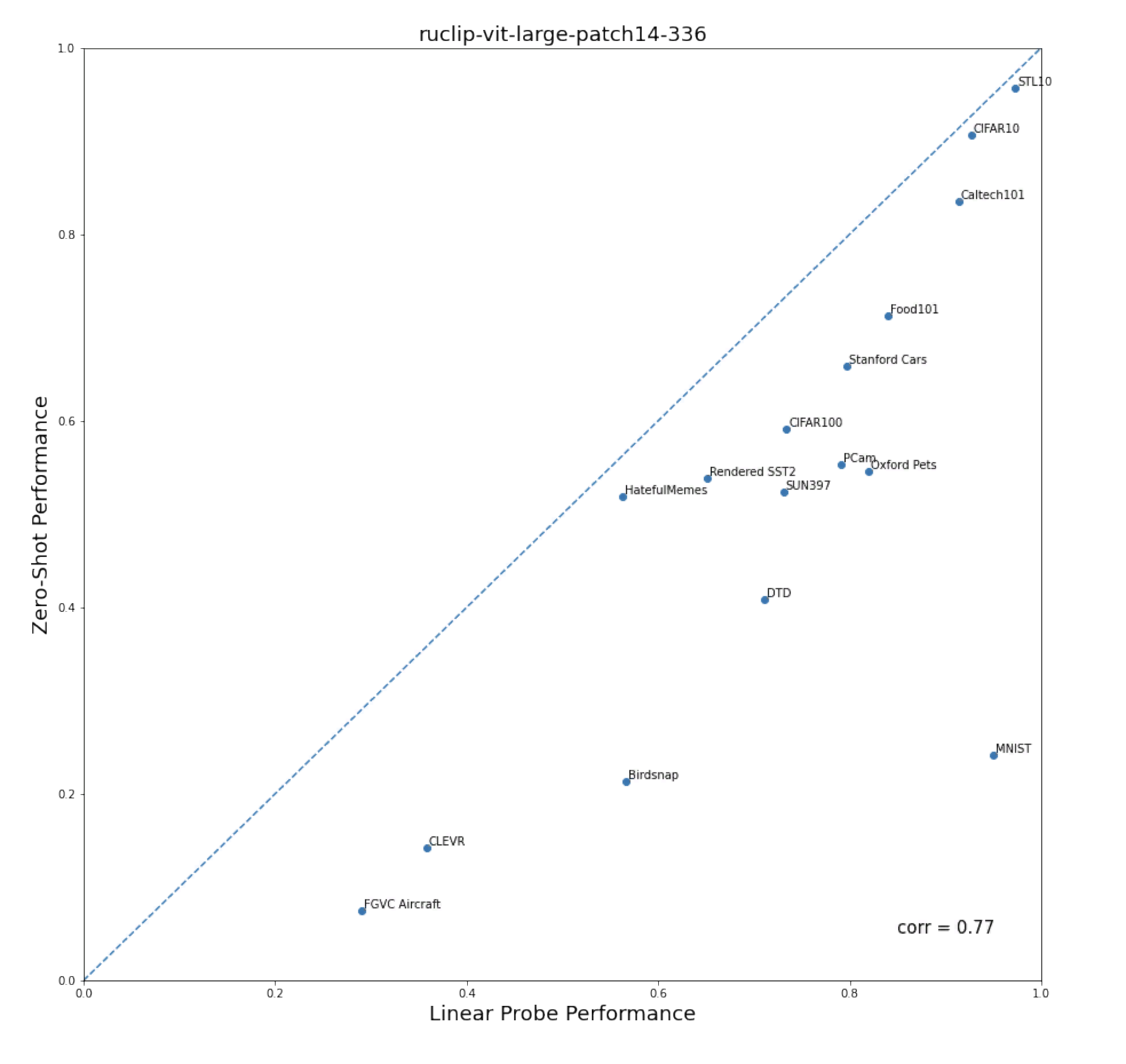
We have evaluated the performance zero-shot image classification on the following datasets:

Dataset	ruCLIP Base [vit-base-patch32-224]	ruCLIP Base [vit-base-patch16-224]	ruCLIP Large [vit-large-patch14-224]	ruCLIP Base [vit-base-patch32-384]	ruCLIP Large [vit-large-patch14-336]	ruCLIP Base [vit-base-patch16-384]	CLIP [vit-base-patch16-224] original + OPUS-MT	CLIP [vit-base-patch16-224] original
Food101, acc	0.505	0.552	0.597	0.642	0.712💥	0.689	0.664	0.883
CIFAR10, acc	0.818	0.810	0.878	0.862	0.906💥	0.845	0.859	0.893
CIFAR100, acc	0.504	0.496	0.511	0.529	0.591	0.569	0.603💥	0.647
Birdsnap, acc	0.115	0.117	0.172	0.161	0.213💥	0.195	0.126	0.396
SUN397, acc	0.452	0.462	0.484	0.510	0.523💥	0.521	0.447	0.631
Stanford Cars, acc	0.433	0.487	0.559	0.572	0.659💥	0.626	0.567	0.638
DTD, acc	0.380	0.401	0.370	0.390	0.408	0.421💥	0.243	0.432
MNIST, acc	0.447	0.464	0.337	0.404	0.242	0.478	0.559💥	0.559
STL10, acc	0.932	0.932	0.934	0.946	0.956	0.964	0.967💥	0.970
PCam, acc	0.501	0.505	0.520	0.506	0.554	0.501	0.603💥	0.573
CLEVR, acc	0.148	0.128	0.152	0.188	0.142	0.132	0.240💥	0.240
Rendered SST2, acc	0.489	0.527	0.529	0.508	0.539💥	0.525	0.484	0.484
ImageNet, acc	0.375	0.401	0.426	0.451	0.488💥	0.482	0.392	0.638
FGVC Aircraft, mean-per-class	0.033	0.043	0.046	0.053	0.075	0.046	0.220💥	0.244
Oxford Pets, mean-per-class	0.560	0.595	0.604	0.587	0.546	0.635💥	0.507	0.874
Caltech101, mean-per-class	0.786	0.775	0.777	0.834	0.835💥	0.835💥	0.792	0.883
Flowers102, mean-per-class	0.401	0.388	0.455	0.449	0.517💥	0.452	0.357	0.697
Hateful Memes, roc-auc	0.564	0.516	0.530	0.537	0.519	0.543	0.579💥	0.589

And for linear-prob evaluation:

Dataset	ruCLIP Base [vit-base-patch32-224]	ruCLIP Base [vit-base-patch16-224]	ruCLIP Large [vit-large-patch14-224]	ruCLIP Base [vit-base-patch32-384]	ruCLIP Large [vit-large-patch14-336]	ruCLIP Base [vit-base-patch16-384]	CLIP [vit-base-patch16-224] original
Food101	0.765	0.827	0.840	0.851	0.896💥	0.890	0.901
CIFAR10	0.917	0.922	0.927	0.934	0.943💥	0.942	0.953
CIFAR100	0.716	0.739	0.734	0.745	0.770	0.773💥	0.808
Birdsnap	0.347	0.503	0.567	0.434	0.609	0.612💥	0.664
SUN397	0.683	0.721	0.731	0.721	0.759💥	0.758	0.777
Stanford Cars	0.697	0.776	0.797	0.766	0.831	0.840💥	0.866
DTD	0.690	0.734	0.711	0.703	0.731	0.749💥	0.770
MNIST	0.963	0.974💥	0.949	0.965	0.949	0.971	0.989
STL10	0.957	0.962	0.973	0.968	0.981💥	0.974	0.982
PCam	0.827	0.823	0.791	0.835	0.807	0.846💥	0.830
CLEVR	0.356	0.360	0.358	0.308	0.318	0.378💥	0.604
Rendered SST2	0.603	0.655	0.651	0.651	0.637	0.661💥	0.606
FGVC Aircraft	0.254	0.312	0.290	0.283	0.341	0.362💥	0.604
Oxford Pets	0.774	0.820	0.819	0.730	0.753	0.856💥	0.931
Caltech101	0.904	0.917	0.914	0.922	0.937💥	0.932	0.956
HatefulMemes	0.545	0.568	0.563	0.581	0.585💥	0.578	0.645

Also, we have created speed comparison based on CIFAR100 dataset using Nvidia-V100 for evaluation:

	ruclip-vit-base-patch32-224	ruclip-vit-base-patch16-224	ruclip-vit-large-patch14-224	ruclip-vit-base-patch32-384	ruclip-vit-large-patch14-336	ruclip-vit-base-patch16-384
iter/sec	308.84 💥	155.35	49.95	147.26	22.11	61.79

Authors

Alex Shonenkov: Github, Kaggle GM
Daniil Chesakov: Github
Denis Dimitrov: Github
Igor Pavlov: Github
Andrey Kuznetsov: Github
Anastasia Maltseva: Github

ai-forever/ru-clip