Flow Free Solver

team :

abd-Elrahman ragab hashem
Abd-Allah Khaled Kamal
Saleh Mahmoud Saleh

Supervisor: Dr. Mahmoud Atef

table of content

- team:
table of content
Flow Free Solver
problem formulation
Dumb algorithm
- Totally random
  - Results for dump
- Next free variable
  - Results
    - Totally random
    - First free variable
Smart Algorithm
optimization
bonus work for bigger maps
Smarter solver
Graphical Results
Reference

Flow Free Solver

A solver for Flow Free puzzles using back tracking search for CSPs.

The problem

Boards are typically a square grid with any number of colors to connect. A well-designed board (an assumption made by this solver) has a unique solution, and requires the entire board to be filled in without any "zig-zagging" paths. A consequence of being an NP-complete puzzle is that, although solutions can be verified quickly, there is no known efficient algorithm to find a solution, and the time required to solve the problem increases very quickly as the board size grows. How do we leverage a computer to quickly find the solution to a given board? We can devise a metric to score potential paths towards the solution, and we investigate the paths that maximize this function first.

Getting started

From terminal

cd ./src
python main_dumb.py # for the dumb heuristic
python main_smart.py # for the smart heuristic
python main_smarter.py # for the directional based

Graphical

# It is recommended to create a separate environment before you install the requirements
pip install -r requirements.txt
cd ./src
python app.py

Approaches

These are approaches we took to solve these puzzles, few notes need to be taken before reading. We consider the map as matrix where each element in this matrix is a variable and these variables are coordinates in xy plan, where y grows downwards starting from the top left corner. Assignments are stored in a dictionary-styled data structure where keys are coordinates and values are colors for each coordinate, we use uppercase letters for terminals and lowercase for pipes.

problem formulation

variables

for the map input there are (MxN) variables each one indicate

the color for it's box for the dump and smart solution
the direction of movement in smarter solution

domains

color based approach (dump/smart)

each variable is of type character and can take value as representing the color of it the value can be _ , lower case character or upper case character and values itself depend on map for example in 5x5

B__RO
___Y_
__Y__
_RO_G
_BG__

available value are ['_','b','r','o','y','g'] for each free variable
each terminal has domain of value equal to its color,

example (0,0) has domain ['B'] here is an example for first five variables in 5X5

variable	domain
(0 0)	['B']
(0 1)	['_','b','r','o','y','g']
(0 2)	['_','b','r','o','y','g']
(0 3)	['_','b','r','o','y','g']
(0 4)	['R']
(0 5)	['O']

worth noting here we didn't use numerical representation so we can make the formulas easier to write and debug as formulas became smaller and their number reduced

our approach may be converted to numerical by creating MxN variable for each color with domain [0,1]

Constraints

These are the procedures we took to check the consistency of any new assignments.

Is_good_combination

What we mean by good combination here the state of the selected assignment don't/won't cause any problems. we can wrap them up in the following points

Number of free neighbors >= 2 => true
Number of similar neighbors == 1 and Number of similar neighbors == 1 => true
Number of similar neighbors == 2 and not(is surrounding square filled) => true
Otherwise => false

those constains are implemented easly for example for varialbe (0 1) in 5x5 map the first constrain would be with neighbors x_1_1 and x_0_2

Implies(x_0_1 == 'b', OR(
    x_1_1 == '_') + (x_0_2 == '_') == 2,
    And(x_1_1 == '_')==1 ,(x_0_2 == 'b')==1),
    (x_1_1 == 'b') + (x_0_2 == 'b') == 2))
    )

and same implies for other colors and neighbor variables

despite being complex but we can easily check this constrain using a for loop and if condition here is python code for it

    comb_points_of_interest = [current_assignment_coord]
    comb_points_of_interest.extend(
        get_neighbors_coords(current_assignment_coord,len(inp),len(inp[0])))
    for coord in comb_points_of_interest:
        if is_empty(assignments, coord) or assignments[coord].isupper():
            continue
        good_comb = check_for_good_combinations(
            coord, assignments[coord], assignments, inp)
        if not good_comb:
            return False

    return True

Is_neighbors_terminals_have_valid_path

Checks weather or not any neighboring terminal in locked out, in other word if our newly assigned var : value causes any problem.

Is_terminal_connected

Use the cached on demand updated terminals to check if the same value terminals are already connected, because if so, it doesn't make sense to assign that value to a variable again

Dumb algorithm

For dumb algorithm we used 2 alternative approuches for picking the random variable, totally random variable and the next free variable.

Totally random

Picking a random value and random variable each time check whether or not this assignment is consultant. If it was consistent move to the next assignment in a DFS-styled backtracking.

Results for dump

map	time	Number of hits
5x5	7 ms	443
7x7	+24hrs	???
...	? ms	???

Next free variable

as seen in previous result the total random gave very long run times, so we tried the next dumpiest thing. by just takeing same order as the map, and surpassingly we got some great results .

so the order is:

For free variables pick the first one as next variable starting from (0,0)

map	time	Number of hits
5x5	2 ms	124
7x7	7 ms	452
8x8	200 ms	15695
9x9	80 ms	6208
10x10 1	200 ms	13396
10x10 2	3 s	255112
12x12	158 s	12903209
12x14	5hr 16min	1548384192
14x14	+24hrs	???

Results

Totally random

5x5:

map ../input/input55.txt solution time = 0.005998373031616211 sec
map ../input/input55.txt number of hits = [443] 
BrrRO
bryYo
brYoo
bROoG
bBGgg

7x7 and higher:

TimeOut! more than (24hrs)

First free variable

5x5:

map ../input/input55.txt solution time = 0.002267599105834961 sec
map ../input/input55.txt number of hits = [124] 
BrrRO
bryYo
brYoo
bROoG
bBGgg

7x7:

map ../input/input77.txt solution time = 0.007232666015625 sec
map ../input/input77.txt number of hits = [452] 
gggOooo
gBggGYo
gbbBRyo
gyyYryo
gyrrryo
gyRyyyo
GyyyOoo

8x8

map ../input/input88.txt solution time = 0.20182538032531738 sec
map ../input/input88.txt number of hits = [15695] 
yyyRrrGg
yBYPprrg
yboOpGRg
yboPpggg
ybooooYy
ybbbBOQy
yQqqqqqy
yyyyyyyy

9x9

map ../input/input991.txt solution time = 0.0804746150970459 sec
map ../input/input991.txt number of hits = [6208] 
DbbBOKkkk
dbOooRrrk
dbRQqqQrk
DBrrrrrrk
gGkkkkkkk
gkkPppppG
gkYyyyYpg
gkkkkkKPg
ggggggggg

10x10 1

map ../input/input10101.txt solution time = 0.22327589988708496 sec
map ../input/input10101.txt number of hits = [13396] 
RGgggggggg
rrrrOoooOg
yYPrQqqqQg
ypprrrrrrg
ypGgbbbbrg
yppgbrRbrg
yypgbrBbrg
Pypgbrrrrg
pYpgbbbbBg
pppggggggg

10x10 2

map ../input/input10102.txt solution time = 3.133574962615967 sec
map ../input/input10102.txt number of hits = [255112] 
tttppppppp
tBtpfffffp
tbTPFBTVfp
tbbbbbtvfp
tttttttvfP
Fnnnnnnvff
fnssssnvvf
fnSNHSNHvf
fnnnhhhhVf
ffffffffff

12x12

map ../input/input1212.txt solution time = 148.92762875556946 sec
map ../input/input1212.txt number of hits = [12903209] 
kkkkkkkkkkkk
kooooooooook
kokkkKyYgGok
kokYyyyGgook
kOkPpoooooQk
kkkRpOQqqqqk
rrrrPaARKkkk
rDddDaWrrrrr
raaaaawwwwWr
raBbbbbbbbBr
raaaaaaaaaAr
rrrrrrrrrrrr

12x14

map ../input/input1214.txt solution time = 18969.79822649236564258 sec
map ../input/input1214.txt number of hits = [1548384192] 
pppPkkkkkkkK
pggGkggGaaaA
pgkkkgPaaYyY
pgkqQgpaBbbb
pgKqggpADddb
pggqgNpDOodB
ppgqgnpddodd
WpgQgnppdoRd
wpgggnNpdord
wpppppppdord
wwwwwwwWdord
dddddddddOrd
dRrrrrrrrrrd
dddddddddddd

Smart Algorithm

Using a combination of helping heuristics and approaches that can be controlled via config dict in src/algorithms/smart.py including MRV to chose the next variable, LCV for choosing the value, Degree Heuristics as a tie breaker and Weak locker these heuristic are "togglable" due to optimization issues, check optimization labeled PRs for more information.

used combination:

Forward checking
MRV (minimum remaining value)
Degree heuristic
Least constraining value

forward checking

find domain for variables
if variable has zero domain
return case failure

def forward_check(variables_domain):
    for coords in variables_domain:
        if len(variables_domain[coords]) == 0:
            return False
    return True

Results

5x5

results

without forward_check

map time Number of hits

5x5 7 ms 443
with forward_check

map time Number of hits

5x5 9 ms 28

map	time	Number of hits
5x5	9 ms	28

MRV

find domain for variables
choose variables with smallest domain
implementation pseudo code

    smallest_domain = math.inf
    selected_coords = []
    for coord in variables_domain:
        domain_len = len(variables_domain[coord])
        if domain_len < smallest_domain:
            selected_coords = []
            smallest_domain = domain_len

        if smallest_domain == domain_len:
            selected_coords.append(coord)

    return selected_coords

initial results *

map	time (s)
7x7	1.87
8x8	1.73
9x9	6.87
10x10	?.??

optimization

limitation

variable domain calculation increase with map size
- example
  - 14x14 every time calculate domain
    for (196 - terminals) variable
- solution
  - update only constrained variables
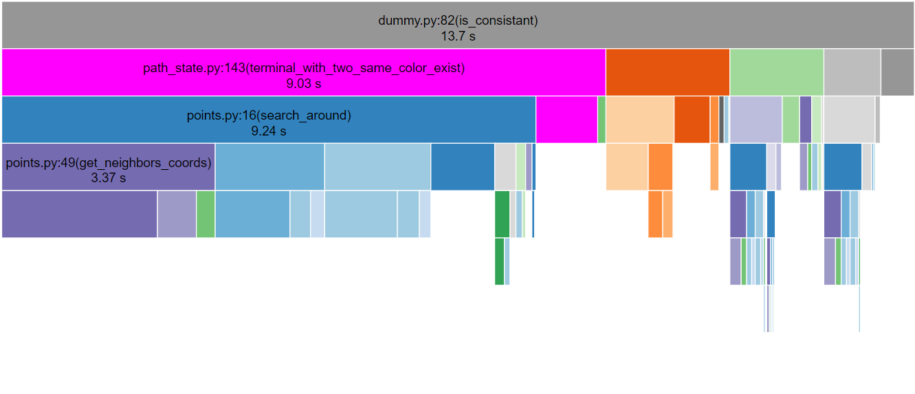
consistency check represent the bottleneck

improvement in constrains

profile for 991

terminal constrain was checking every terminal has only on path

update

check only neighbor terminals this improved performance significantly

profile for 991

results

map	time (s)
7x7	0.085
8x8	0.157
9x9	0.858
10x10(1)	3.300
10x10(2)	1.680
12x12	14.971
12x14	??.???

lazy surrounding squares

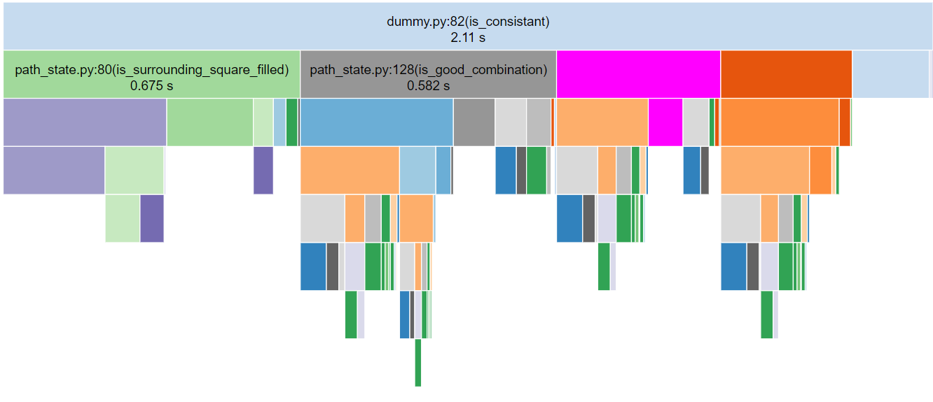
check surrounding squares "zigzag" only when have 2 same color neighbors. Because if we have a good combination we are in one of these two cases

only one free neighbor and same color neighbor (no squares)
only 2 or more free neighbors (no squares)

implementation

def check_for_good_combinations(coord, current_color, assignments, inp):
    empty_neighbors = search_around(coord, inp, assignments, is_empty)
    if len(empty_neighbors) >= 2:
        return True
    same_color_neighbors = get_same_color_neighbors(
        coord, current_color, assignments, inp)
    if len(same_color_neighbors) == 2:
        # we don't need is surrounding square anywhere but here
        ssf = is_surrounding_square_filled(assignments,inp,coord)
        return not ssf
    if len(empty_neighbors) == 1 and len(same_color_neighbors) == 1:
        return True
    return False

Results

map	time (s)
10x10(1)	2.26
10x10(2)	1.09
12x12	8.72
12x14	??.???

Cache connected terminals

We can cache connected terminals to quickly check whether or not the selected value is consistent
Using a shared object between backtracks that gets updated only when a variable is consistent

Implementation

Inside backtrack

if is_consistant(initial_state, {var: value},  assignments, inp, connected_terminals):
    before_assgen_connected_terminal = connected_terminals
    refreshed_connected_terminals = refresh_connected_terminals( {var: value}, assignments, connected_terminals, initial_state, inp)

Results

map	time (s)
10x10(1)	1.49
10x10(2)	0.728
12x12	5.38
12x14	??.???

bonus work for bigger maps

dynamic domain-upgrade

save variable domain
only update constrained variables

the constrained variables

are empty neighbor (point good combination)
are empty neighbor for occupied neighbor
(point neighbors/terminal combination)
every point when terminal is connected (terminal connected)

implementation

variables_domain = {}
connection_changed = len(connected_terminals)>len(prev_connected_terminal)
first_run = prev_variable == None
if connection_changed or first_run:
    # update all variables
    for coord in variables:
        domain = get_available_domain(coord,
        assignments,connected_terminals)
        variables_domain[coord] = domain
else:
    variables_domain = pickle.loads(pickle.dumps(prev_domain))
    del variables_domain[prev_variable]
    big_neighbors = get_constrained_neighbors(prev_variable,inp,assignments )
    for coord in big_neighbors:
        domain = get_available_domain(coord, assignments, inp,connected_terminals)
        variables_domain[coord] = domain
return variables_domain

results

map	time	Number of hits
5x5	6 ms	17
7x7	16 ms	41
8x8	30 ms	52
9x9 (1)	57 ms	67
10x10 (1)	189 ms	320
10x10(2)	93 ms	139
12x12	290 ms	331
12x14	193 ms	148
14x14	7875 ms	10309

degree heuristic

use as tie breaker
choose variable that constrain others implementation

most_constraining_count = -math.inf
for coord in variables:
    constrained_count = len(
        get_constrained_neighbors(coord,inp, assignments))
    if constrained_count > most_constraining_count:
        most_constraining_count = constrained_count
        most_constraining_var = coord
return most_constraining_var

results

didn't improve
made heuristic optional

least constraining value

choose value that doesn't affect domains

implementation

count_value_ordered = []
for value in domain:
    updated_variable_domains = get_available_domain_multiple(
        {**{coord: value}, **assignments}, inp, coord,)
    count_constrained = 0
    
    for coord in updated_variable_domains:
        if len(updated_variable_domains[coord]) < len(variables_domain[coord]):
            count_constrained += 1

    count_value_ordered.append((count_constrained, value))
count_value_ordered.sort()
order_domain_values = []
for count, value in count_value_ordered:
    order_domain_values += value

return order_domain_values

results

map	time	Number of hits
5x5	5 ms	17
7x7	16 ms	56
8x8	23 ms	52
9x9 (1)	65 ms	100
10x10 (1)	166 ms	330
10x10(2)	240 ms	482
12x12	838 ms	1178
12x14	163 ms	146
14x14	2230 ms	2374

Best Smart results

5x5

map ../input/input55.txt solution time = 0.005002737045288086 sec
map ../input/input55.txt number of hits = [17] 
BrrRO
bryYo
brYoo
bROoG
bBGgg

7x7

map ../input/input77.txt solution time = 0.01697063446044922 sec
map ../input/input77.txt number of hits = [56] 
gggOooo
gBggGYo
gbbBRyo
gyyYryo
gyrrryo
gyRyyyo
GyyyOoo

8x8

map ../input/input88.txt solution time = 0.023000001907348633 sec
map ../input/input88.txt number of hits = [52] 
yyyRrrGg
yBYPprrg
yboOpGRg
yboPpggg
ybooooYy
ybbbBOQy
yQqqqqqy
yyyyyyyy

9x9

map ../input/input991.txt solution time = 0.06594991683959961 sec
map ../input/input991.txt number of hits = [100] 
DbbBOKkkk
dbOooRrrk
dbRQqqQrk
DBrrrrrrk
gGkkkkkkk
gkkPppppG
gkYyyyYpg
gkkkkkKPg
ggggggggg

10x10 1

map ../input/input10101.txt solution time = 0.16699814796447754 sec
map ../input/input10101.txt number of hits = [330] 
RGgggggggg
rrrrOoooOg
yYPrQqqqQg
ypprrrrrrg
ypGgbbbbrg
yppgbrRbrg
yypgbrBbrg
Pypgbrrrrg
pYpgbbbbBg
pppggggggg

10x10 2

map ../input/input10102.txt solution time = 0.24605417251586914 sec
map ../input/input10102.txt number of hits = [482] 
tttppppppp
tBtpfffffp
tbTPFBTVfp
tbbbbbtvfp
tttttttvfP
Fnnnnnnvff
fnssssnvvf
fnSNHSNHvf
fnnnhhhhVf
ffffffffff

12x12

map ../input/input1212.txt solution time = 0.8389444351196289 sec
map ../input/input1212.txt number of hits = [1178] 
kkkkkkkkkkkk
kooooooooook
kokkkKyYgGok
kokYyyyGgook
kOkPpoooooQk
kkkRpOQqqqqk
rrrrPaARKkkk
rDddDaWrrrrr
raaaaawwwwWr
raBbbbbbbbBr
raaaaaaaaaAr
rrrrrrrrrrrr

12x14

map ../input/input1214.txt solution time = 0.16399812698364258 sec
map ../input/input1214.txt number of hits = [146] 
pppPkkkkkkkK
pggGkggGaaaA
pgkkkgPaaYyY
pgkqQgpaBbbb
pgKqggpADddb
pggqgNpDOodB
ppgqgnpddodd
WpgQgnppdoRd
wpgggnNpdord
wpppppppdord
wwwwwwwWdord
dddddddddOrd
dRrrrrrrrrrd
dddddddddddd

14x14

map ../input/input1414.txt solution time = 2.230055093765259 sec
map ../input/input1414.txt number of hits = [2374] 
oooowwwwwkkkkk
oBbowAaawkpppk
oobowwWawkpRPk
DobooAaaWkprkk
dobboooOBkprkG
dOYbbbbbbKprkg
ddyyyyyyyDprkg
Gdddddddydprkg
grrrrrRdYdprkg
grqqqqQdddprkg
grqpppppppprkg
grQPrrrrrrrrkg
grrrrKkkkkkkkg
gggggggggggggg

Smarter solver

This is the final optimization.

In this part, we tried a totally different approach that is more efficient than all past approaches because it offers an excellent constraints propagation technique (arc consistency). We used directions as a domain for all variables instead of colors. So we have 6 different directions:

variables = all empty squares in HxW input matrix (Xij) where ‘i = y-index & j = x-index’
domain = {'└', '┌', '│', '┘', '─', '┐'}

we had also assistant variables (colors : Cij, domain: input colors) used to check that the same colors sources are connected but in some simple cases (like 5x5 map) there is no need of them

all border variables have special domains, four corner variables have one value domain and other border variable have 3 values domain.

domain[(0, 0)] = {'┌'}
domain[(h-1, 0)] = {'└'}
domain[(h-1, w-1)] = {'┘'}
domain[(0, w-1)] = {'┐'}
domain[(0, i)] = {'┌', '┐', '─'}
domain[(i, 0)] = {'└', '┌', '│'}
domain[(h-1, i)] = {'└', '┘', '─'}
domain[(i, w-1)] = {'┐', '┘', '│'}
domain[(i, j)] = {'└', '┌', '│', '┘', '─', '┐'}

constraints:

there are a lot of assignment constraints. We will put here some examples of them, the rest of constraints are in the code and can be deducted also.

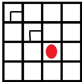
1-If there is a square Xij that had value '┘' , then its upper square Xi-1,j (if it is not source square) must have the value '│', otherwise there will be a zigzag. This can be formed in pseudo-code:

constraint_1 = [ Implies(Xij == '┘' , THEN: Xi-1,j = '│' ]

2- If there is a square Xij that had value '┘' , then its left square Xi,j-1 (if it is not source square) must have the value '─', otherwise there will be a zigzag. This can be formed in pseudo-code:

constraint_2 = [ Implies(Xij == '┘'  , THEN:  Xi-1, j  = '─' ]

3- If there f there is a square Xij that had value '│' , then its upper square Xi-1,j (if it is not source square) must NOT have the values '─', '┘', '└' otherwise there will be a cross in the path. This can be formed in pseudo-code:

constraint_3 = [ Implies(Xij == '│' , THEN: Xi-1, j  != '─' AND Xi-1, j  != '┘' AND Xi-1, j  != '└' ]

if(is_in_domain[(i-1, j)]):
            delete_corner(inp, ['┘', '└'], (i-1, j), domains,
                          Num_of_domain_values, domain_levels, assigns)
            reduce_domain(['─'], (i-1, j), domains,
                          Num_of_domain_values, domain_levels, assigns)

Sources constraints:

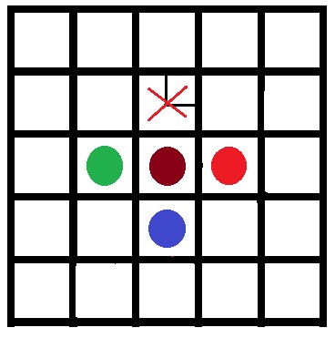
every source have at most 4 neighbors (up , down, right, left) and it must be connected to one of them. For example: if the right, left and down squares of a source are also sources, then its upper square must have value of '┌', '│' and '┐'. so it must NOT have a value of '┘' or '─' or '└'.

if(len(terminal_domain[terminal]) == 1):
            direction = terminal_domain[terminal]

            if(direction == 'UP'):
                delete_corner(inp, ['┘', '└'], (i-1, j), domains, Num_of_domain_values, domain_levels, [])
                reduce_domain(['─'], (i-1, j), domains, Num_of_domain_values, domain_levels, [])

Improvement of performance:

we can improve the performance by using two things:

1- constraint propagation (arc consistency):

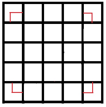
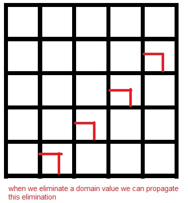
there are some squares that are related together. For example : if the upper left corner had the value ‘┌’ then its lower right square must have the same value. Otherwise there will be a zigzag or cross. This continues until hitting a color source square:

so if we know that some value is wrong for some variable and we removed it from this variable domain, then it should remove it from related squares also:

2- colored sources relations:

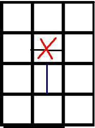
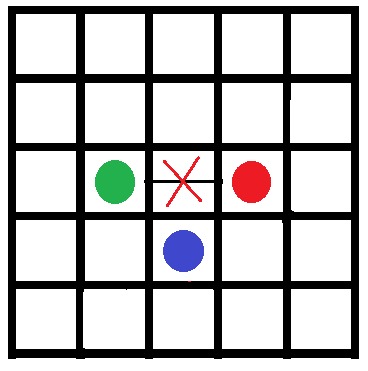
if there is two sources having DIFFERENT colors and can be connected with one line, then we could remove this line from domain:

#xij is a terminal where I is y index and j is x index
if((is_in_terminals[(i, j+2)]) and (color[i][j+2] != color[i][j]) and is_in_empty_squares[(i, j+1)]):
reduce_domain(['─'], (i, j+1), domains, Num_of_domain_values, domain_levels)

Implementation:

we firstly look for the least domain length variables (that have one value in its domain) and then we start assigning the variables that have two values in domain. We used depth first recursion and backtrack. So we have a TWO branching-factor recursion (Binary tree). This is an excellent branching factor compared to other ways. We used a heuristic values that is corner value for border squares {'└', '┌', '┘', '┐'} and straight lines {'─', '│'} otherwise.

def backtrack(inp, terminals, terminal_domain, domains, Num_of_domain_values, domain_levels, assigns, colors, is_in_domain, is_in_terminals):

    if(len(assigns) == len(domains)):
        return assigns

    _terminal_domain = copy.deepcopy(terminal_domain)
    _domains = copy.deepcopy(domains)
    _Num_of_domain_values = copy.deepcopy(Num_of_domain_values)
    _domain_levels = copy.deepcopy(domain_levels)
    _assigns = copy.deepcopy(assigns)
    _colors = copy.deepcopy(colors)

    location, direction = get_heuristic(inp, _domain_levels[1], _domains)

    _domain_levels[1].remove(location)

    Assign(inp, direction, location, terminals, _terminal_domain, _domains, _Num_of_domain_values,
           _domain_levels, _assigns, _colors, is_in_domain, is_in_terminals)

    is_consistant = apply_arc_consistency(inp, terminals, _terminal_domain, _domains,
                                          _Num_of_domain_values, _domain_levels, _assigns, _colors, is_in_domain, is_in_terminals)

    if(is_consistant):
        res = backtrack(inp, terminals, _terminal_domain, _domains, _Num_of_domain_values,
                        _domain_levels, _assigns, _colors, is_in_domain, is_in_terminals)
        if(res != False):
            return res

    domains[location].remove(direction)
    dire = min(domains[location])
    domain_levels[1].remove(location)

    Assign(inp, dire, location, terminals, terminal_domain, domains, Num_of_domain_values,
           domain_levels, assigns, colors, is_in_domain, is_in_terminals)

    iss_consistant = apply_arc_consistency(inp, terminals, terminal_domain, domains,
                                           Num_of_domain_values, domain_levels, assigns, colors, is_in_domain, is_in_terminals)

    if(iss_consistant):
        _res = backtrack(inp, terminals, terminal_domain, domains, Num_of_domain_values,
                         domain_levels, assigns, colors, is_in_domain, is_in_terminals)
        if(_res != False):
            return _res

    return False

Advantages of using directions approach instead of colors approach:

in some smaller maps(5x5) all variables are initially assigned , so we didn’t need recursion for this map.
in the worst case (biggest map : 14x14) there was about 47% of variables assigned initially and this is a very good result that reduced the unkown variables size to almost half.
the branching factor (2) is very small compared to color-approach (using colors some times causes a branching factor of 7 or 8.

Smarter Solver Results

Map	time	Number of assignments(hits)
5X5	0.4 ms	15
7x7	0.8 ms	39
8x8	0.7 ms	50
9x9	1.8 ms	75
10x10(1)	2.9 ms	102
10x10(2)	3 ms	126
12x12	5.7 ms	177
12x14	5.8 ms	186
14x14	6.6 ms	193

5x5:

Result: 

B┌─RO
││┌Y│
││Y┌┘
│RO┘G
└BG─┘
---------------------------------
map ../input/input55.txt solution time = 0.0004048347473144531 sec
number of variables:  39

7x7:

Result: 

┌─┐O──┐
│B└─GY│
│└─BR││
│┌─Y│││
││┌─┘││
││R┌─┘│
G└─┘O─┘
---------------------------------
map ../input/input77.txt solution time = 0.0008220672607421875 sec

8x8:

Result: 

┌─┐R─┐G┐
│BYP┐└┐│
││┌O│GR│
│││P┘└─┘
││└──┐Y┐
│└──BOQ│
│Q────┘│
└──────┘
---------------------------------
map ../input/input88.txt solution time = 0.0007193088531494141 sec

9x9

Result: 

D┌─BOK──┐
││O─┘R─┐│
││RQ──Q││
DB└────┘│
┌G┌─────┘
│┌┘P───┐G
││Y───Y││
│└────KP│
└───────┘
---------------------------------
map ../input/input991.txt solution time = 0.0018935203552246094 sec

10x10 1

Result: 

RG───────┐
└──┐O───O│
┌YP│Q───Q│
│┌┘└────┐│
││G┐┌──┐││
│└┐││┌R│││
└┐││││B┘││
P││││└──┘│
│Y││└───B│
└─┘└─────┘
---------------------------------
map ../input/input10101.txt solution time = 0.002902984619140625 sec

10x10 2

Result: 

┌─┐┌─────┐
│B││┌───┐│
││TPFBTV││
│└───┘││││
└─────┘││P
F┌────┐│└┐
││┌──┐│└┐│
││SNHSNH││
│└─┘└──┘V│
└────────┘
---------------------------------
map ../input/input10102.txt solution time = 0.003052949905395508 sec

12x12

Result: 

┌──────────┐
│┌────────┐│
││┌──K┌Y┌G││
│││Y──┘G┘┌┘│
│O│P┐┌───┘Q│
└─┘R│OQ───┘│
┌──┘P┌ARK──┘
│D──D│W└───┐
│┌───┘└───W│
││B───────B│
│└────────A│
└──────────┘
---------------------------------
map ../input/input1212.txt solution time = 0.005738496780395508 sec

12x14

Result: 

┌──P┌──────K
│┌─G│┌─G┌──A
││┌─┘│P┌┘Y─Y
│││┌Q│││B──┐
││K│┌┘│AD─┐│
│└┐││N│DO┐│B
└┐│││││└┐│└┐
W││Q││└┐││R│
││└─┘└N│││││
│└─────┘││││
└──────W││││
┌───────┘O││
│R────────┘│
└──────────┘
---------------------------------
map ../input/input1214.txt solution time = 0.005768537521362305 sec

14x14 Result:

┌──┐┌───┐┌───┐
│B┐││A─┐││┌─┐│
└┐││└─W││││RP│
D││└┐A─┘W│││┌┘
││└┐└──OB││││G
│OY└────┘K││││
└┐└─────┐D││││
G└─────┐││││││
│┌────R│Y│││││
││┌───Q└─┘││││
│││┌──────┘│││
││QP┌──────┘││
│└──┘K──────┘│
└────────────┘
---------------------------------
map ../input/input1414.txt solution time = 0.006555795669555664 sec

results comparsion

time

Map	time (dump)	time(smart)	time(smarter)
5X5	2 ms	5 ms	0.4 ms
7x7	7 ms	16 ms	0.8 ms
8x8	200 ms	23 ms	0.7 ms
9x9	80 ms	65 ms	1.8 ms
10x10(1)	200 ms	166 ms	2.9 ms
10x10(2)	3 s	240 ms	3 ms
12x12	158 s	838 ms	5.7 ms
12x14	5hr 16min	163 ms	5.8 ms
14x14	-	2230 ms	6.6 ms

number of hits

Map	Number of assignments(dump)	Number of assignments(smart)	number of assignments(smarter)
5X5	124	17	15
7x7	452	56	39
8x8	15695	52	50
9x9	6208	100	75
10x10(1)	13396	330	102
10x10(2)	255112	482	126
12x12	12903209	1178	177
12x14	1548384192	146	186
14x14	-	2374	193

Graphical Results

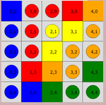
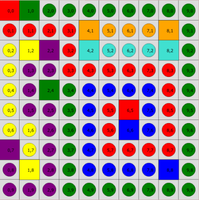
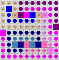
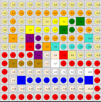
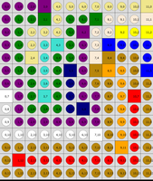
5x5:

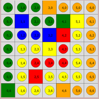
7x7

8x8

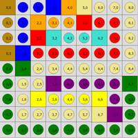
9x9

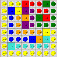
10x10 1

10x10 2

12x12

12x14

14x14

Reference

Russell, S. J. (2016). Artificial intelligence: A modern approach. Harlow: Pearson.

ak-seyam/FlowFree

Flow Free Solver

team :

table of content

Flow Free Solver

The problem

Getting started

From terminal

Graphical

Approaches

problem formulation

variables

domains

color based approach (dump/smart)

Constraints

Dumb algorithm

Totally random

Results for dump

Next free variable

Results

Totally random

First free variable

Smart Algorithm

forward checking

Results

results

MRV

initial results *

optimization

limitation

improvement in constrains

update

results

lazy surrounding squares

implementation

Results

Cache connected terminals

Implementation

Results

bonus work for bigger maps

dynamic domain-upgrade

the constrained variables

results

degree heuristic

results

least constraining value

results

Best Smart results

Smarter solver

constraints:

there are a lot of assignment constraints. We will put here some examples of them, the rest of constraints are in the code and can be deducted also.

Sources constraints:

Improvement of performance:

we can improve the performance by using two things:

1- constraint propagation (arc consistency):

2- colored sources relations:

Implementation:

Advantages of using directions approach instead of colors approach:

Smarter Solver Results

results comparsion

time

number of hits

Graphical Results

Reference