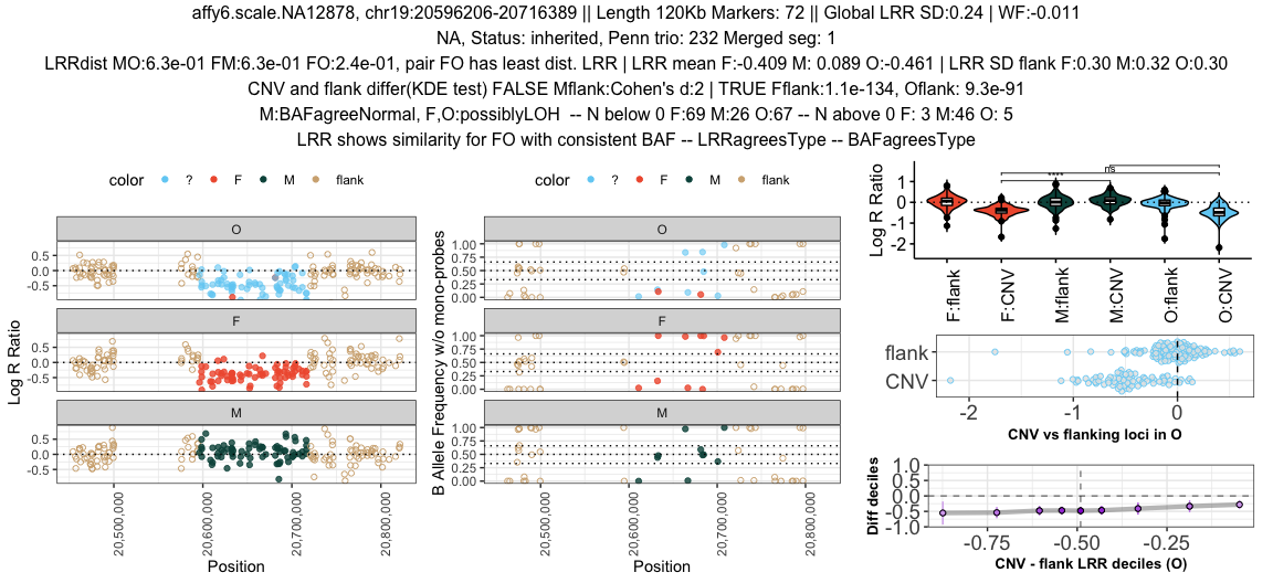
SeeCiTe is a novel CNV quality control tool that post-processes output from current CNV calling tools exploiting child-parent trio data to classify calls in quality categories and provide a set of visualizations for each putative CNV call in the offspring. It utilizes probe-level CNV data in trios (and singletons) to systematically highlight potential artefacts and visualize signal intensities in a streamlined fashion suitable for biobank scale studies.
This vignette describes all steps necessary to run SeeCiTe analysis, using the public HapMap trio data, with intermidiate outputs supplied with the package for the:
Make sure the dependencies are installed fist:
generic_packages <- c("magrittr", "dplyr", "tidyr", "tools", "purrr", "utils", "rlang", "bedr")
plotting_packages <- c("ggplot2", "scales", "gridExtra", "cowplot", "rogme", "ggpubr")
stat_packages <- c("statip", "outliers", "effsize", "lawstat", "ks")
packages <- c(generic_packages, plotting_packages, stat_packages)

if (length(setdiff(packages, rownames(installed.packages()))) > 0) {
  install.packages(setdiff(packages, rownames(installed.packages())))
}

library(devtools)
devtools::install_github('davetang/bedr')
devtools::install_github("GRousselet/rogme")
Use devtools package to install directly from GitHub (by default it will force the upgrade of the installed packages, which might be undesirable, then set dependencies to FALSE):
devtools::install_github("aksenia/SeeCiTe", dep = FALSE)The preparation step takes in 1) an original PennCNV-trio output (produced by running PennCNV’s detect_cnv.pl with the -trio flag) and 2) merged and/or filtered by frequency and size file in a standard PennCNV format (PennCNV’s clean_cnv.pl will do the segment merging automatically and output a file in such format). The merged file defines the CNVs to analyse in terms of boundaries and loci covered, e.g. all CNVs that are in the first file but do not overlap with the CNVs in the second file will be ignored.
The function runExtractInheritance will take these two input files and produce additional intermediate files, necessary for consequent steps, shown below, with the prefix of the merged file:
# Loading SeeCiTe
library(SeeCiTe)
# PennCNV-trio output
file_original <- system.file("extdata", "affy6ceu.original.triocnv", package = "SeeCiTe")
# PennCNV merge output
file_merged <- system.file("extdata", "affy6ceu.merged.filtered.triocnv", package = "SeeCiTe")
# Input files for SeeCiTe
input_files <- runExtractInheritance(filename_orig = file_original, filename_merged = file_merged)
The input files now contain CNVs to analyse for each offspring and inheritance, decoded from PennCNV-trio HMM state. The merging log is also created to keep track whether a CNV was merged and if so, how many segments were merged.
print(input_files)
# $triocnv_file
# [1] "SeeCiTe/inst/extdata/affy6ceu.merged.filtered_annot_offspring.triocnv"
#
# $merge_trace
# [1] "SeeCiTe/inst/extdata/affy6ceu.merged.filtered_merge.log"
dir <- dirname(file_original)
# Intermidiate files for the reference of inheritance mapping.
list.files(dir, pattern = tools::file_path_sans_ext(basename(file_merged)), full.names = F)
# [1] "affy6ceu.merged.filtered.triocnv"
# [2] "affy6ceu.merged.filtered_annot.triocnv"
# [3] "affy6ceu.merged.filtered_annot_offspring.triocnv"
# [4] "affy6ceu.merged.filtered_merge.log"
# [5] "affy6ceu.merged.filtered_unmaskedstatus.triocnv"For the extraction of the SNP-level data for each individual in a trio the following inputs are needed: 1) PFB file (same file with probe coordinates used when running PennCNV); 2) full path to PennCNV installation; 3) File with paths to LRR and BAF signal files in a tab-separated format in the order father, mother, offspring (same as in PennCNV-trio); 4) A parameter setting how many probes in flanks to extract; 5) dataset name - it must be consistent and will be used for file naming throughout the project; 6) full path to the directory in which the extracted SNP data will be stored, for each CNV (must be created in advance).
pfb_file <- file.path("~/Documents/uib/dev/toydata/affygw6.hg19.sorted.pfb")
penn_path <- "~/local/PennCNV1.0.4"
penn_trio_list <- file.path("~/Documents/uib/dev/toydata/affy6hm_trio.tab")
n_flanking_snp <- 5
run_dir <- "~/Documents/uib/dev/toydata/dev"

commands <- makePythonCommands(penn_path=penn_path,
                               pfb_file=pfb_file,
                               penn_trio_list=penn_trio_list,
                               triocnv_file=input_files[["triocnv_file"]],
                               n_flanking_snp=5,
                               dataset="affy6ceu",
                               run_dir=run_dir)
print(commands)
# $cnv
# [1] "python3 SeeCiTe/inst/python/extract_snp_cnv.py -l ~/Documents/uib/dev/toydata/affy6hm_trio.tab -c SeeCiTe/inst/extdata/affy6ceu.merged.filtered_annot_offspring.triocnv -d affy6ceu -p ~/Documents/uib/dev/toydata/affygw6.hg19.sorted.pfb -s ~/local/PennCNV1.0.4 -o ~/Documents/uib/dev/toydata/dev"
#
# $flank
# [1] "python3 SeeCiTe/inst/python/extract_snp_flanks.py -l ~/Documents/uib/dev/toydata/affy6hm_trio.tab -c SeeCiTe/inst/extdata/affy6ceu.merged.filtered_annot_offspring.triocnv -d affy6ceu -p ~/Documents/uib/dev/toydata/affygw6.hg19.sorted.pfb -s ~/local/PennCNV1.0.4 -o ~/Documents/uib/dev/toydata/dev -f 5"
The result will be two script files with one line per CNV with a command for PennCNV infer_snp_allele.pl that will do the extraction, terminating by lines that collect the data into one table for the whole cohort. This must be run by the user. For large cohorts one can split the commands into batches or submit to a cluster.
The previous step extracts SNP data into files in the provided run_dir: files with prefix probecoord.txt, snp_flank.txt and snp_cnv.log. The main CNV file is triocnv_file in input_data object, while merge_trace is the merging log in the same object. Finally, cnv_qcsum_file is the QC summary output of PennCNV. The cache_id tells where R should store cache for core calculations.
args <- list(triocnv_file=input_files[["triocnv_file"]],
             probecoord_file=system.file("extdata", "affy6ceu.probecoord.txt", package = "SeeCiTe"),
             snp_flank_file=system.file("extdata", "affy6ceu.snp_flank.txt", package = "SeeCiTe"),
             snp_cnv_log_file=system.file("extdata", "affy6ceu.snp_cnv.log", package = "SeeCiTe"),
             cnv_qcsum_file=system.file("extdata", "affy6ceu.qcsum", package = "SeeCiTe"),
             dataset="affy6ceu",
             cache_id="~/Documents/uib/dev/toydata",
             merge_trace=input_files[["merge_trace"]])
Now all inputs are in order and can be read and formatted:
main_dt <- readInputs(args = args)
# [1] "Reading merged formatted PennCNV trio file for offspring SeeCiTe/inst/extdata/affy6ceu.merged.filtered_annot_offspring.triocnv"
# [1] "Reading probes file SeeCiTe/inst/extdata/affy6ceu.probecoord.txt"
# [1] "Collapsing duplicate probes"
# [1] "Annotating probes in CNV loci"
# [1] "Reading extracted intensity for flanking regions SeeCiTe/inst/extdata/affy6ceu.snp_flank.txt"
#
#    denovo inherited
#         6        43
# [1] "Reading denovo test results for CNV regions SeeCiTe/inst/extdata/affy6ceu.snp_cnv.log"
# [1] "Reading quality summary file SeeCiTe/inst/extdata/affy6ceu.qcsum"
# [1] "Reading merging log file SeeCiTe/inst/extdata/affy6ceu.merged.filtered_merge.log"
candidateCnvs <- main_dt[["data"]]First, a summary statistic collection step, for each CNV in offspring:
clu_baf <- runAnalyzeSignal(input_data = candidateCnvs, args = args, use_cache = T)
# [1] "Found cached file ~/Documents/uib/dev/toydata/affy6ceu_clu_baf.rds, reading in"
head(clu_baf[,c(1:4)], n=3)
# # A tibble: 3 x 4
#   cnvTypeBAF    relation nprobes33_66 nprobes_cn4
#   <chr>         <chr>           <int>       <int>
# 1 F:possiblyLOH F                   0           0
# 2 M:possiblyLOH M                   0           0
# 3 O:possiblyLOH O                   0           0
The clasification is the final step in the analysis which annotates each CNV with suggested inheritance and SeeCiTe quality class.
cnv_class <- classifyTrios(clu_baf)
with(cnv_class, table(seecite, inheritanceTest))
#             inheritanceTest
# seecite      denovo inherited mosaic unclear
#   borderline      3         0      3      19
#   probable        0        18      0       0
# unlikely 3 3 0 0The results can be visualized either for each single CNV region or for a whole cohort:
Sample <- "affy6.scale.NA12878"
Cnv <- "chr19:20596206-20716389"
plotRawTrio(input_data = candidateCnvs %>% dplyr::filter(sample==Sample, coordcnv==Cnv),
            sifted_data = clu_baf %>% dplyr::filter(sample==Sample, coordcnv==Cnv),
            penn_qcsum = main_dt[["qcsum"]] %>% dplyr::filter(sample==Sample),
            merge_trace = main_dt[["merge"]] %>% dplyr::filter(sample==Sample, coordcnv==Cnv))
This will write a pdf file with such plots per SeeCiTe category:
plotCohort(main_data=main_dt,
           sifted_data=clu_baf,
           classified_data=cnv_class,
           output_dir = "~/Documents/uib/dev/toydata/affy6ceu_viz",
           dataset="affy6ceu",
           subset_nprobes=20,
           subset_length=150000)
Finally, the summary statistics and SeeCiTe classifications can be written out as plain text files, together with bed (UCSC 6-column style) and plink formatted CNV regions:
writeSeecite(classified_data=cnv_class,
          output_dir = "~/Documents/uib/dev/toydata/affy6ceu_viz",
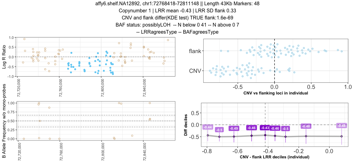
dataset="affy6ceu")The SeeCite core algorithm is based on comparison of intensity distributions between the individuals in a trio. However there is a number of individual-level metrics that can be useful out of trio context. We extended the tool functionality to process the single samples data and calculate these metrics. The adapted simplified plotting function is also available.
First step is to extract the signal intensities with a helper script extract_snp_single.py, which takes as input PennCNV format and a sample map (one line per sample, comma-separated, “sampleid,path/to/lrrbaf_file”):
python3 extract_snp_single.py -c data/affy6hm.initial_merged.triocnv -m data/samples_map.txt -o data -d SNGL -f 30The output file data/SNGLE.signal_flanks_30.txt (provided with the package sample data) will contain all the information needed for consequent steps:
single_file =  system.file("extdata", "SNGLE.signal_flanks_30.txt", package = "SeeCiTe")
single_data <- readSingle(snp_file = single_file)
head(single_data, n = 2)
# # A tibble: 2 x 13
#   Name    Chr Position locus coordcnv sample copynumber numsnp relation Origin
#   <chr> <int>    <int> <chr> <chr>    <chr>       <int>  <int> <chr>    <lgl>
# 1 AFFX…     6 32412480 flank chr6:32… affy6…          1     18 O        NA
# 2 AFFX…     6 32412480 flank chr6:32… affy6…          1     18 O        NA
# # … with 3 more variables: type <chr>, parameter <chr>, value <dbl>
sclu_baf <- runAnalyzeSignal(single_data,
args = list(cache_id="~/Documents/uib/dev/toydata",
dataset="SNGLE"),
single = T,
use_cache = T)
# [1] "Found cached file ~/Documents/uib/dev/toydata/SNGLE_clu_baf.rds, reading in"
scnv_class <- classifySingles(sclu_baf)
Sample <- "affy6.shelf.NA12892"
Cnv <- "chr1:72768418-72811148"
plotSingle(input_data = single_data %>% dplyr::filter(sample==Sample, coordcnv==Cnv),
sifted_data = sclu_baf %>% dplyr::filter(sample==Sample, coordcnv==Cnv),
print_title = T)To write out multiple plots:
plotCohort(main_data=list(data=single_data),
           sifted_data=sclu_baf,
           classified_data=scnv_class,
           output_dir = "~/Documents/uib/dev/toydata/single_viz",
           dataset="SNGLE",
single = TRUE)If you use this package, please cite “SeeCiTe: a method to assess CNV calls from SNP arrays using trio data”, Ksenia Lavrichenko, Øyvind Helgeland, Pål R Njølstad, Inge Jonassen, Stefan Johansson. Bioinformatics, btab028, doi: https://doi.org/10.1093/bioinformatics/btab028

