This analysis has a small dataset which explores the dataset from application point of view and I hope it would be a precursor to complex analysis using the same or different technique.
Note:
- Microsoft Excel's regression limits to linear regression analysis however one can try to fit with one independent variable or multiple independent variables.
- R2 is R-squared value which is defined as the measure of proprortion of variance of dependent variable explained by the independent variable. The higher the proportion, the better is the relationship between dependent and independent variable/s.
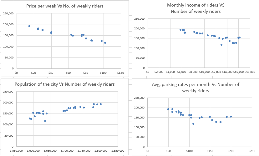
This is a transit demand data set and the dependent variable under consideration is Number of weekly riders and there are four independent variables whose predictability we want to know.
All the scatter plots helps use decide to go for a linear regression model
Assumptions to apply linear regression model:
- There must be a linear relation between independent and dependent variables.
- There should not be any outliers present.
- No heteroscedasticity
- Observations of the error term are uncorrelated with each other. It is called as Auto-correlation.
- Absence of multicollinearity.
- All independent variables are uncorrelated with the error term
- Error terms should be normally distributed with mean 0.
Though it is not an exact linear relation, the whole purpose of modelling is to understand the uncertainty complemented with statistical analysis. Let's apply the regression technique and discover if the assumptions get validated without which our model doesn't stand a suitable fit for the given data and future predictions.
R2 Value = 0.95
While R2 is one parameter to look out for, the most standard way is to check the residual plotst to evaluate the model. The more random the errors are, the better your model. It means you shouldn't be able to form a pattern in any part of the plot as far residuals are concerned.
1. There must be a linear relation between independent and dependent variables.
The first assumption can be validated from the scatter plots and the results of the regression which showcases different coefficients and the fitted values are calculated using the linear equation. Y = β0 + β1X1 + β2X2 + .... + (error)
2. There should not be any outliers present.
The residuals mustn't be more than 3 standard deviations away from the residual mean. Let's check that with a calculation of standardized residuals.
The maximum value is 2.20 standard deviations away from the mean with which we can move ahead.
3. No heteroscedasticity.
This means the residuals must have a constant variance across all the observations. The residual vs fitted values plot tells about it.
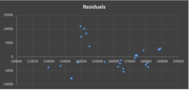
Residual plot for this model:
In our residual plot, the variance fans in which is a sign of heteroscedasticity. A different interpretation is that it can be seen that for fitted values < 140000 of the Number of weekly riders variable, residuals are -ve while they are +ve in between [1400000, 150000]. This made me easy to find out a pattern which is not the desired outcome when checking for goodness of fit via residual plots.
To remove heteroscedasticity (pure), either re-defining the variables or weighted regression technique (How in MS-Excel? - Coming soon) or Dependent variable transformation can be applied and convert the analysis to homscedastic. However, this only matters when understanding the effects of independent variables and not if prediction making is the main goal. Upcoming: Weighted Regression Techniuqe.
Note: To remove impure form of heteroscedasticity, subject-matter expertise is needed as the main concern is finding out the key variables which are reflected in the non-constant variance.
4. Observations of the error term are uncorrelated with each other.
If there is a pattern and one error term (generally the order in which observations are collected) helps in predicting the next error term, then there is problem.
To randomize this serial correlation, independent variables which can be attributed to such effect has to be added and required subject matter expertise. It is out of scope for this analysis as the data set is constrained with respect to the number of independent variables.
5. Absence of multicollinearity.
This means no independent variable is a perfect linear function of other explanatory variables. Just like the case of heteroscedasticity, if predictions are the main goal, evaluating mutlicollinearity can be skipped and I have skipped it. But if interpreting coefficients, p-values are of major concern, then Variance Infation Factor helps in finding out multicollinearity.
6. All independent variables are uncorrelated with the error term.
This has to be taken for granted as there was no precursor information about the data set. And all the given variables were included in the model which lead to a good R2 value (0.95).
7. Error terms should be with mean 0.
It can be seen that the mean of residuals/ error terms is very tiny and can be approximated to 0. This assumption will be however validated as ours is a linear model and we have the constant β0 which takes care of it by forcing the mean of residuals to zero.
In all the required assumptions, multicollinearity and heteroscedasticity are the one which we are uncertain of but as far as predictions are concerned, we can surely ignore the discrepancies with those two assumptions. From a statistical analysis POV, it is highly recommended to dig deep into making this a better model by different solutions offered. Feel free to pitch in if you'd like to perform a deep dive into it. I look forward to working on it as I explore more of the regression analysis technique.
It can be seen from the results of the first model (multiple linear regression - where all the four predictor variables are used), the p-values of all the predictor variable except the price per week are greater than the chosen significance level 0.05. This indicates the relationship between the response variable and the three independent variables - population of the city, monthly income of riders, and average parking rates per month is not really significant. Let's remove those variables for better model precision:
Results of the simple linear regression model (only one predictor variable):
The value of R-squared 0.93 still explains the relationship with the response variable in spite of having only one predictor variable. Basically, we have removed what is not needed which typically happens in real world data sets too.
Now as R-squared value is only useful to some extent to measure goodness of fit (as it a relative measure - %), it doesn't help in assessing the model precision. Model precision is important to build reliable predictive models which can complement decision making. Let's assess the model precision using standard error and compare it to the first model built.
How to know if it is a model with higher precision?
The model with at least 95% of observations nearer to the corresponding fitted line is more precise, i.e., the observed values must be within +/-2*SE.
Standard error of regression for first model (multiple linear regression) = 5406.370168
How many points are close to the fitted line?
It is only one point for which the observed value falls outside the prediction interval of that point. So, there are more than 95% points in this case.
Standard error of regression for second model (simple linear regression) = 5620.113932
How many points are close to the fitted line?
It is only one point for which the observed value falls outside the prediction interval of that point. So, there are more than 95% points in this case too.
Although, it is probable that removing variables with poor/ no relationship with the dependent variables can make the model much more precise. In our case, we can't really distinguish between both of the models for precision as equal number of points are within bounds in their respective fits. This could be due to the scale of the problem (less number of data points in total). It is also observed that the as standard error for the second model (simple linear regression) increased slightly and R2 value decreased slightly which is standard. However, irrespective of the size of changes, they might be practically important based on the business question one wants to answer.
For more complex problems, the precision value to be set is more of a business decision based on how critical the problem is. In that case, we would need more precise models and have to work towards reducing the standard error.


