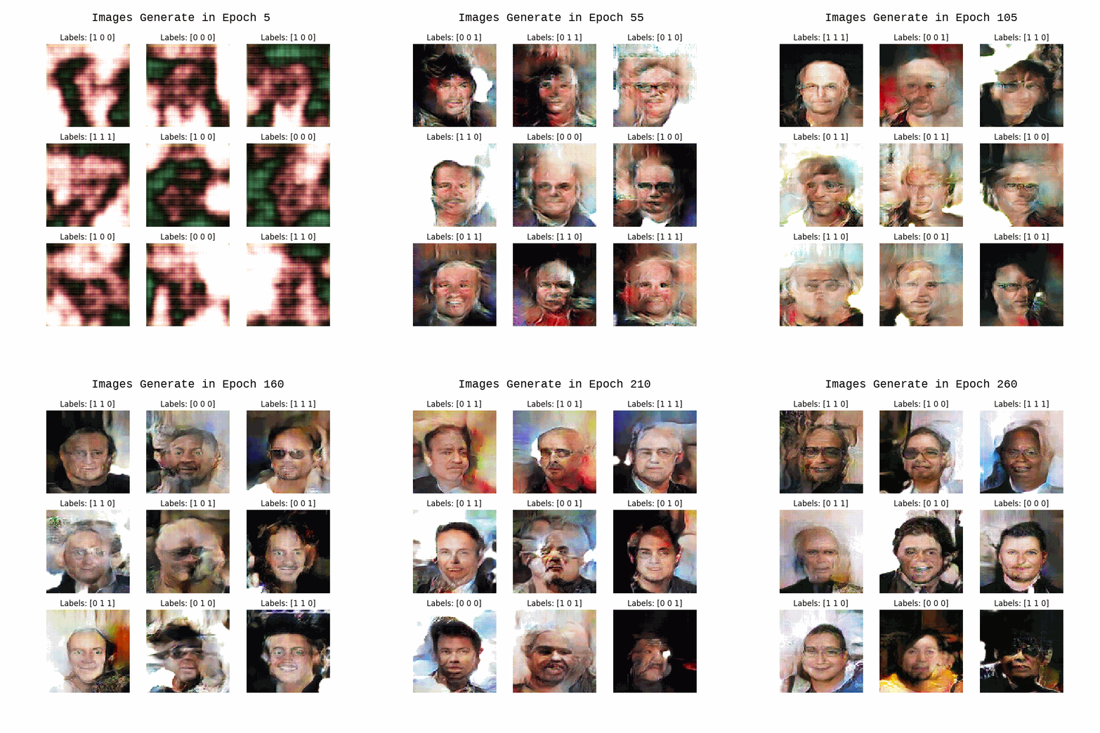
This is the final project of the postgraduate course of Artificial Intelligence with Deep Learning by Universitat Politècnica de Catalunya (UPC). The goal is to build a conditioned GAN that generate faces given some features. To do so, different architectures and known methods have been tested.
This project started on 10th of February of 2020, which implementation occured from 27th of February to 8th of April of 2020.
This network has been implemented with Tensorflow 2.0 and Keras. Experiments were run in Google Colab.
$ git clone https://github.com/anieto95/homogan
$ cd homogan/
$ sudo pip3 install -r requirements.txt
For the whole project, we saved a history of our code source for each experiment. Thus, we decided to simplify code and make it easy to change parameters and experiment with it. For this reason, we created a main framework to experiment.
In order to train the model, parameters should be set in config.json. Once parameters are set, simply run main.py.
Nevertheless, older experiments can be run as well. Source can be found in src/old/ExperimentXX and documents in docs/ExperimentXX. Though parameters can't be changed, they can be tested by running src/old/ExperimentXX/main.py.
If the dataset is not placed in the indicated dataset folder in parameters, the script will automatically download it. Kaggle user and password must be set.
| Parameters | Default value | Notes |
|---|---|---|
| model | src.models.model_15 | Select the model used, different options can be found in src/models. By default it's selected model from Experiment 15, which offers best results. |
| multilabelling | True | Select True if multilabelling is needed, False if not needed. If multilabelling is selected, number of parameters and labels must be selected in Celeba parameters. |
| features | 3 | Number of parameters selected in multilabelling. |
| IMG_HEIGHT | 128 | Height of resized images. |
| IMG_WIDTH | 128 | Width of resized images. |
| Parameters | Default value | Notes |
|---|---|---|
| BUFFER_SIZE | 3000 | Buffer size of dataset. |
| BATCH_SIZE | 100 | Batch size of dataset. |
| kaggleUser | None | Fill Kaggle user in order to download Celeba dataset. |
| kagglePass | None | Fill Kaggle pass in order to download Celeba dataset. |
| dataset_folder | /content/celeba-dataset | Directory where the dataset will be saved. |
| celeba_features | [["Male", 1], ["Eyeglasses"], ["No_Beard"], ["Bald"]] | In order to select filters for the dataset, a list should be included as [FILTER_NAME, VALUE]. In order to selecto features for multilabelling, no value should be included [FEATURE_NAME]. |
| num_img_training | 5000 | Images to be included in the dataset for training. |
| Parameters | Default value | Notes |
|---|---|---|
| latent_dim | 256 | Latent dimension of Input. |
| start_epoch | 0 | If there is a checkpoint loaded, select starting epoch for training. |
| epochs | 100 | Total number of epochs. |
| train_g | 1 | Number of times the generator will be trained. |
| train_d | 1 | Number of times the discriminator will be trained. |
CelebFaces Attributes Dataset (CelebA) is a large-scale face attributes dataset with more than 200K celebrity images, each with 40 attribute annotations. The images in this dataset cover large pose variations and background clutter.
For the whole project, images have been cropped and reduced to 128x128px. For the Experiment 16, images were preprocessed to delete the background.
- Generator (G).
A generative model is a model of the conditional probability of the observable X, given a target y.
- Discriminator (D).
A discriminative model is a model of the conditional probability of the target Y, given an observation x
- Fully Connected (FC).
Fully connected layers connect every neuron in one layer to every neuron in another layer.
- Fully Convolutional (FConv).
The goal is to transform image pixels to pixel categories. Unlike the convolutional neural networks, an FCN transforms the height and width of the intermediate layer feature map back to the size of input image through the transposed convolution layer, so that the predictions have a one-to-one correspondence with input image in spatial dimension.
- Dropout.
At each training stage, individual nodes are either dropped out of the net with probability 1-p or kept with probability p, so that a reduced network is left; incoming and outgoing edges to a dropped-out node are also removed.
- Label Smoothing.
Label smoothing is a regularization technique for classification problems to prevent the model from predicting the labels too confidently during training and generalizing poorly.
- Label Flipping.
Label flipping is a training technique where one selectively manipulates the labels in order to make the model more robust against label noise.
- Batch Normalization.
Batch normalization is a technique for training very deep neural networks that standardizes the inputs to a layer for each mini-batch. This has the effect of stabilizing the learning process and dramatically reducing the number of training epochs required to train deep networks.
- Spectral Normalization.
Spectral Normalization normalizes the spectral norm of the weight matrix W, where the spectral norm σ(W) that we use to regularize each layer is the largest singular value of W. In few words, simply replaces every weight W with W/σ(W).
- Gaussian Noise.
Gaussian Noise is statistical noise having a probability density function equal to that of the normal distribution, which is also known as the Gaussian distribution. In other words, the values that the noise can take on are Gaussian-distributed.
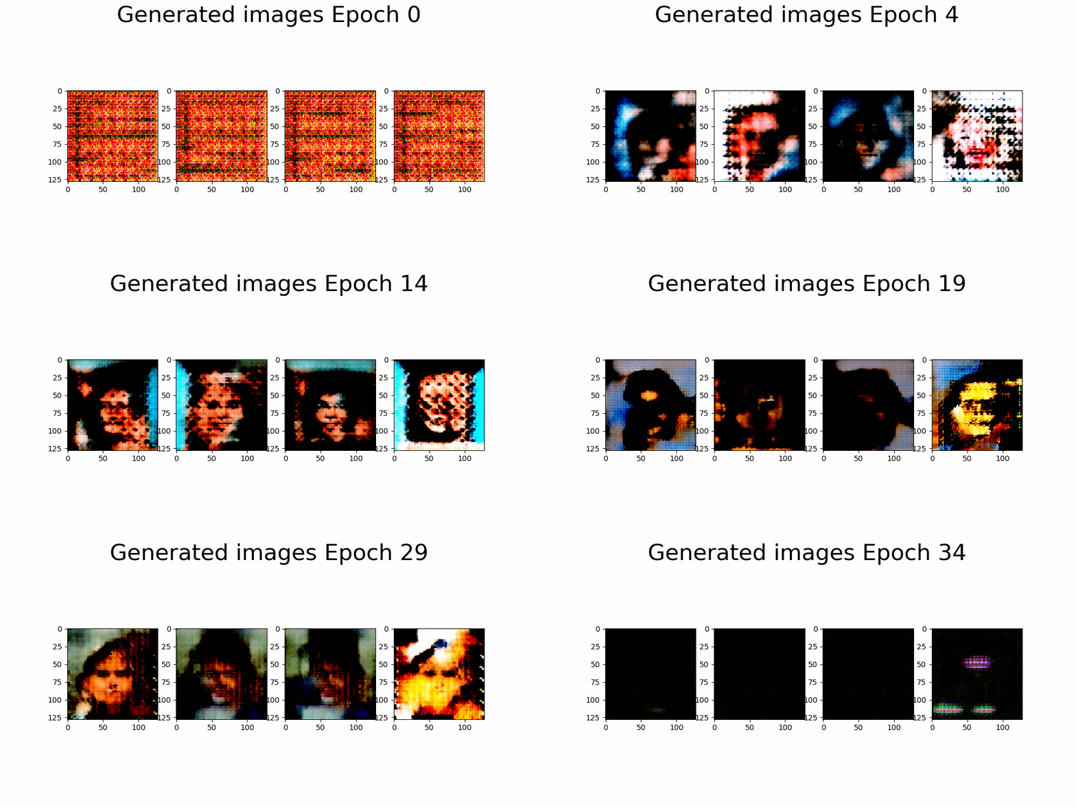
First approach, architecture based on DCGAN.
| Hyperparameters | Observations |
|---|---|
| Trainning size = 10.000 Trainning Epochs = 35 Batch Size = 16 |
* Huge model, generator with over 9M parameters in G vs 400k in the D. * Slow trainning per epoch and high memory consumption. |
| Results GIF |
|---|
 |
Change from previous models:
- Wrap G and D definition in classes.
- Add tensorboard loss tracing.
| Hyperparameters | Observations |
|---|---|
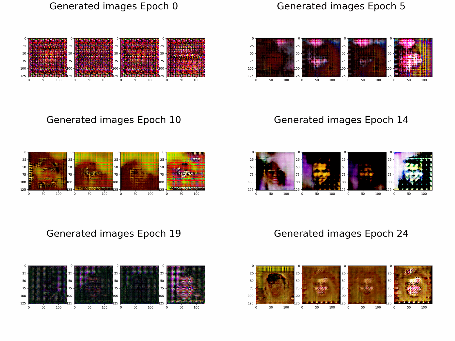
| Trainning size = 10.000 Trainning Epochs = 25 Batch Size = 16 |
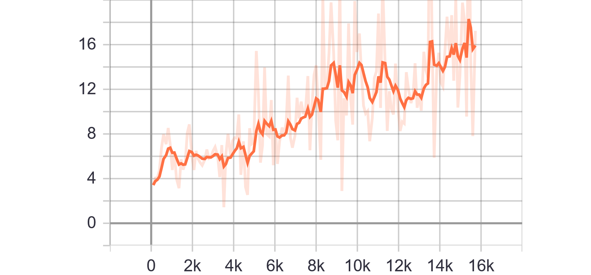
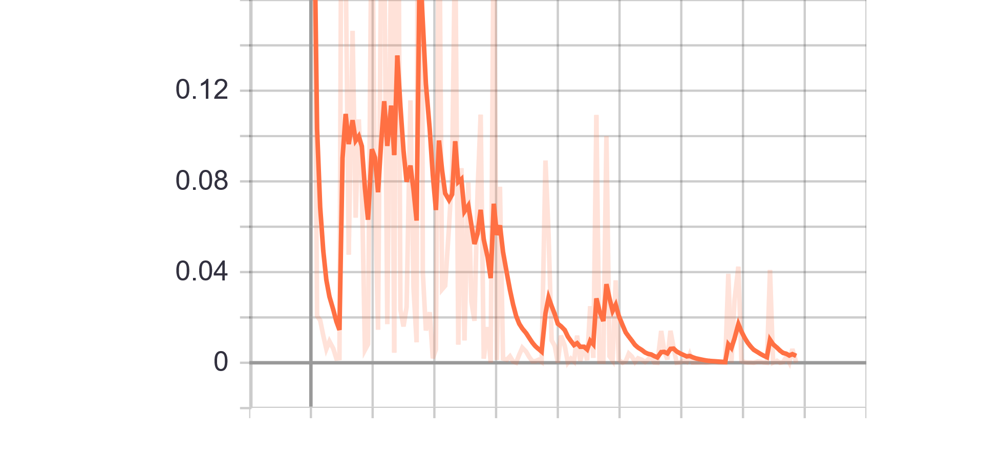
Loss Charts:
 |
 |
|---|---|
| Generator Loss | Discriminator Loss |
| Results GIF |
|---|
 |
Change from previous models:
- Creation of two independent classes for data importing and GAN architecture definition.
- Remove conv layers 1 and 2 from G (reduce number of parameters).
- Remove layer 2 (Conv, BatchNorm, LeackyReLU and Dropout) from D.
- Adde fake and real accuracy metric.
| Hyperparameters | Observations |
|---|---|
| Trainning size = 10.000 Trainning Epochs = 34 Batch Size = 16 |
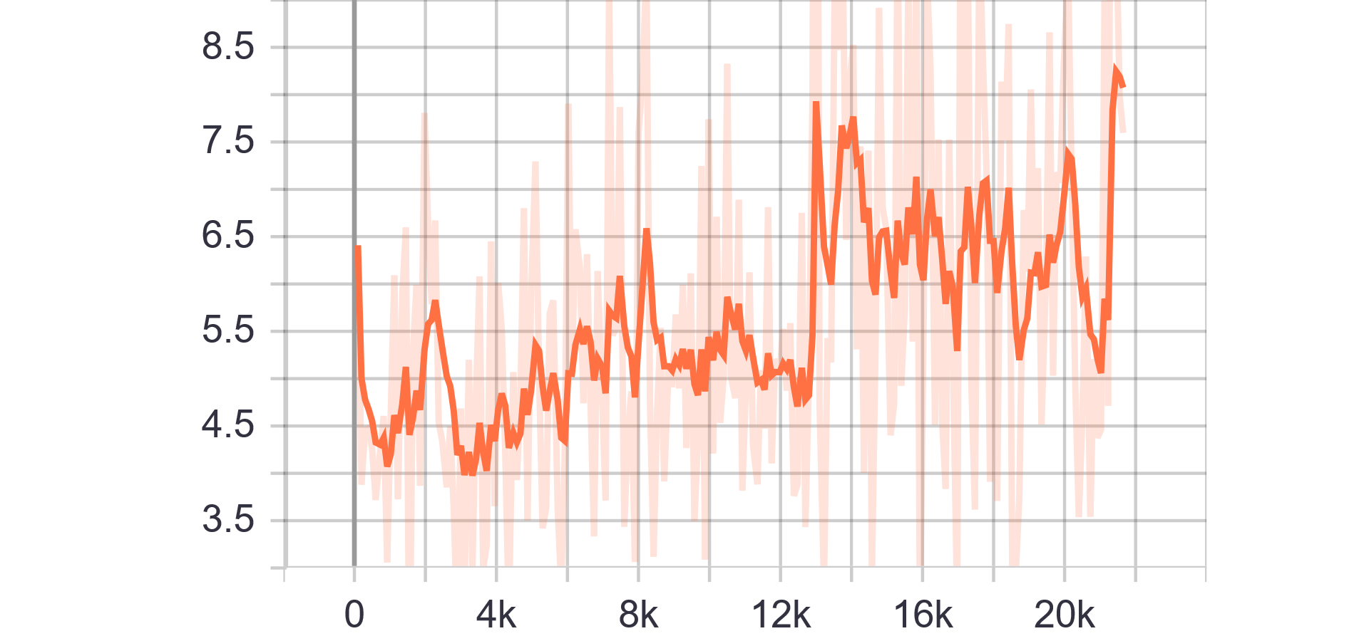
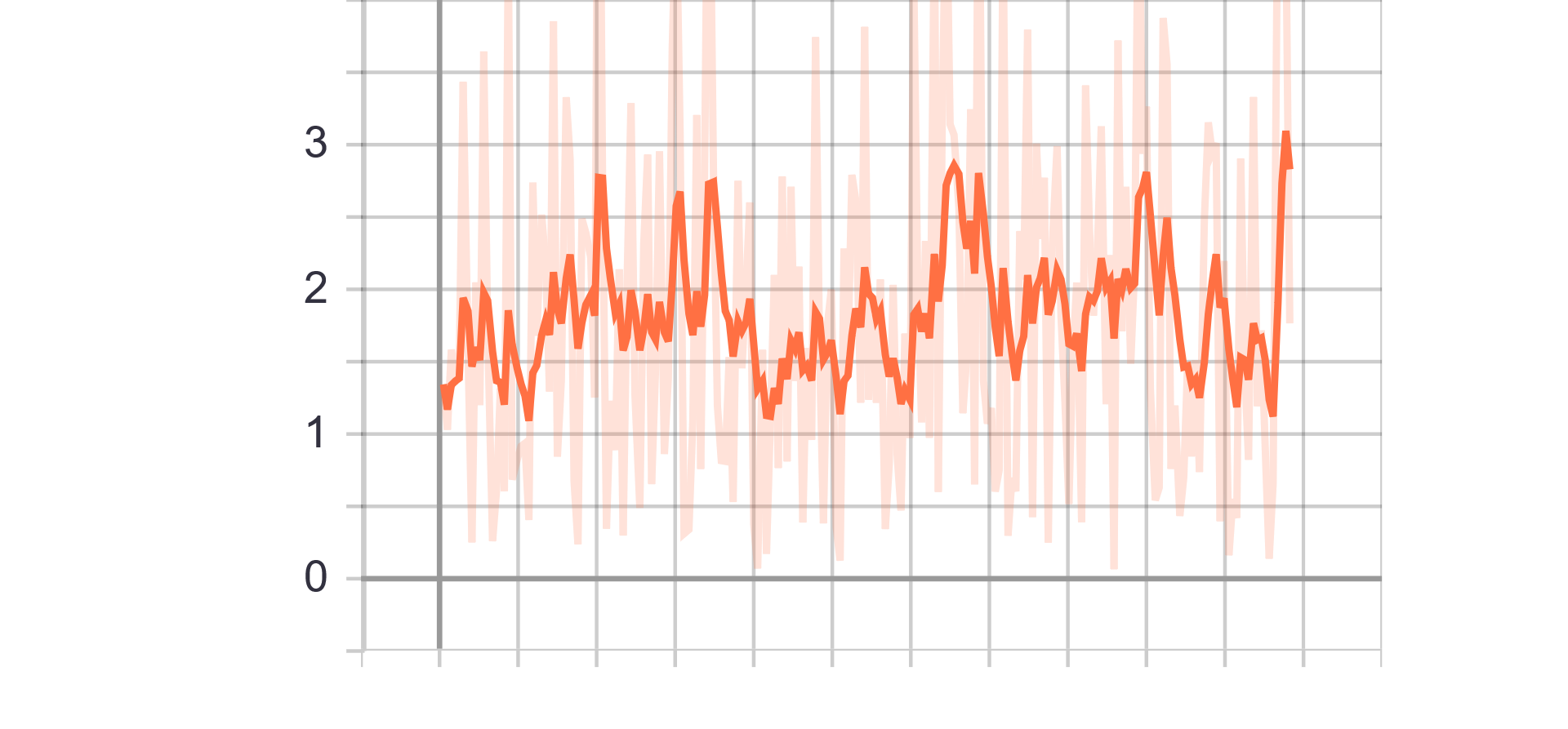
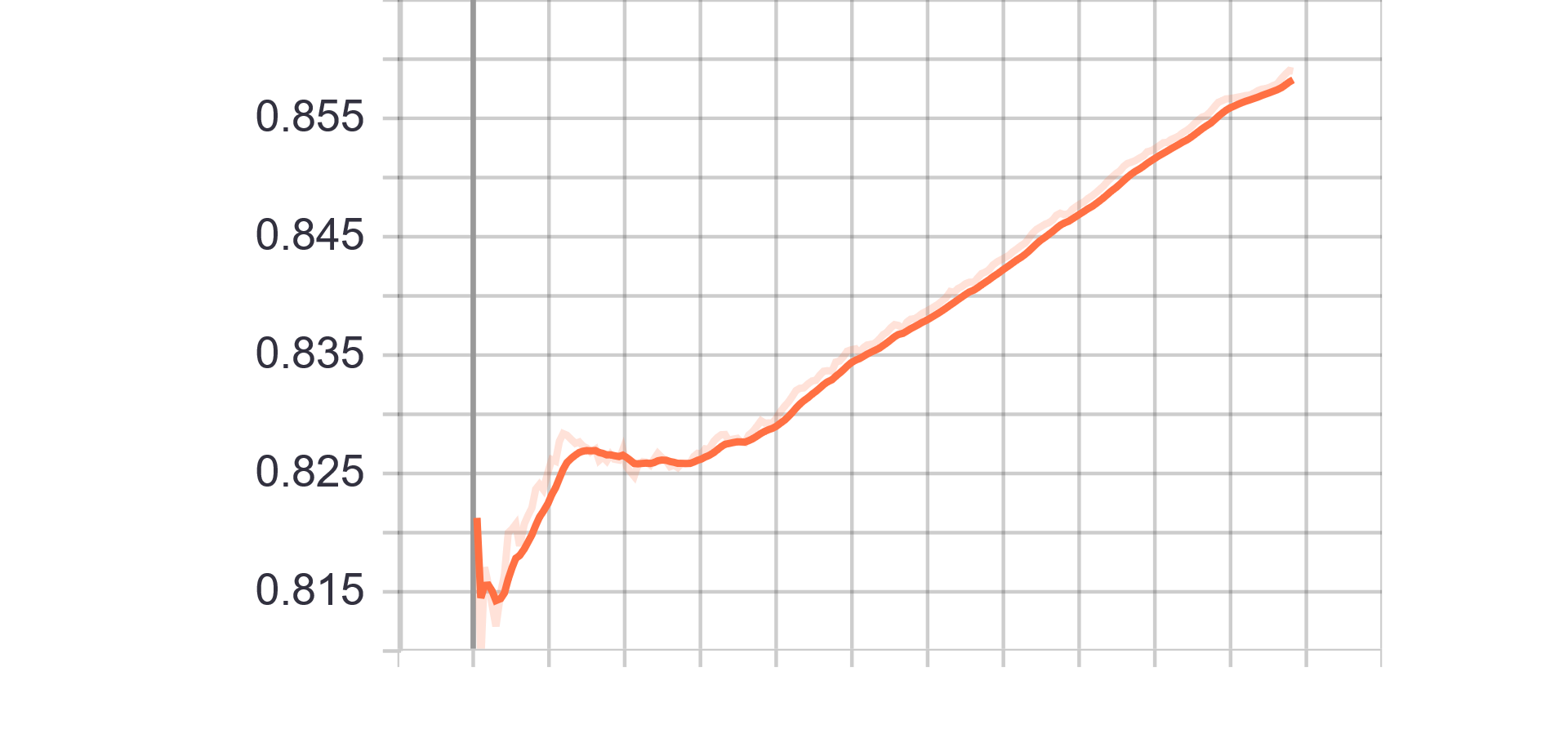
Loss and Accuracy Charts:
 |
 |
|---|---|
| Generator Loss | Discriminator Loss |
 |
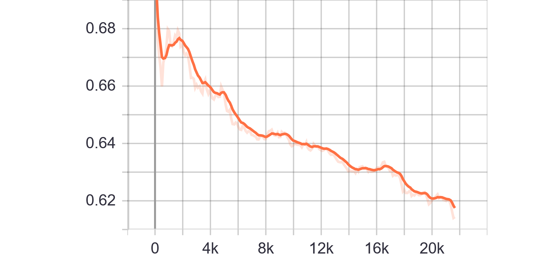 |
| Fake accuracy | Real accuracy |
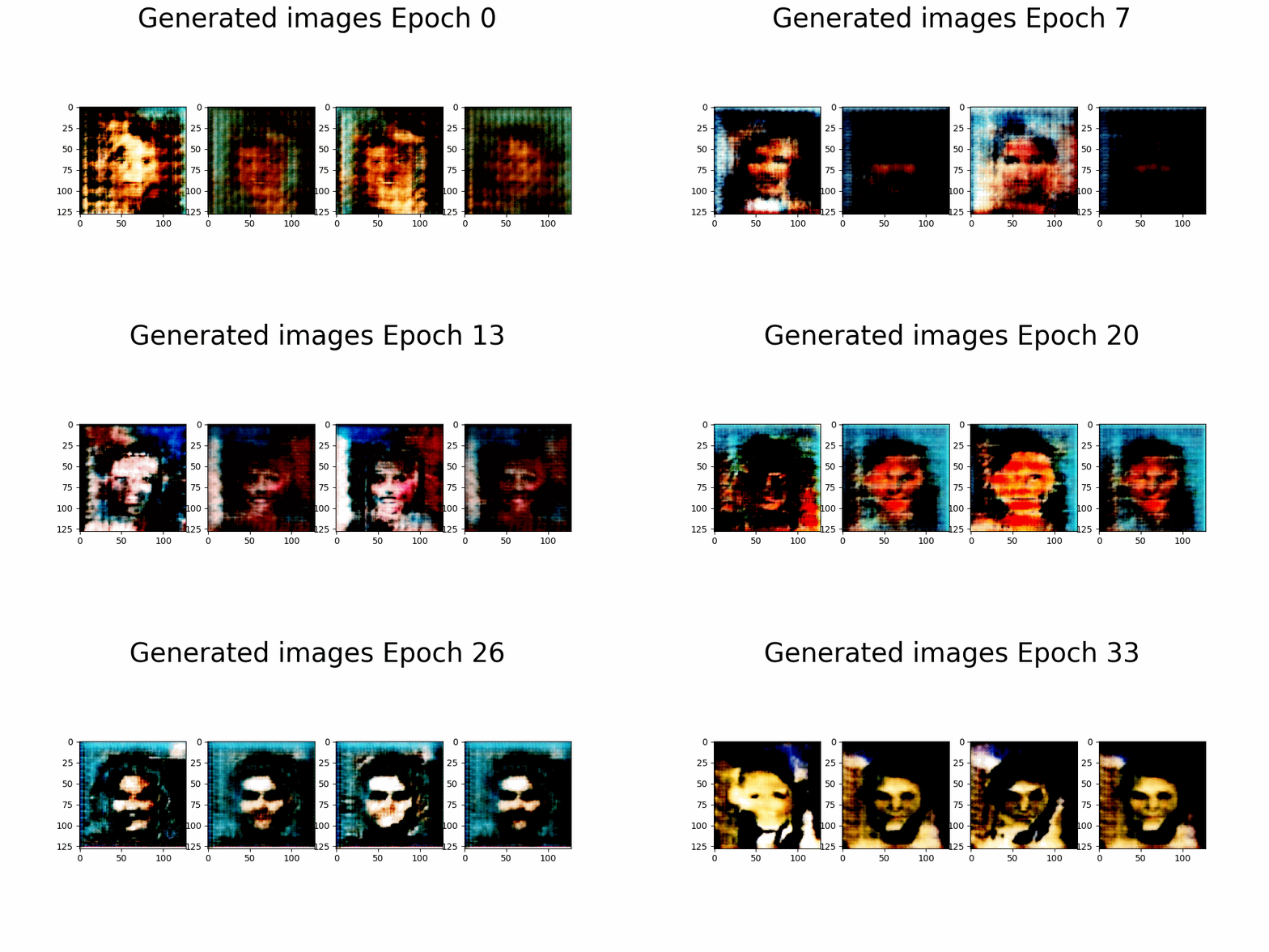
| Results GIF |
|---|
 |
Change from previous models:
- The two FC input layers of the G changed to FConv.
- Update restriction on the D -> D is not updated while G loss is >4.
| Hyperparameters | Observations |
|---|---|
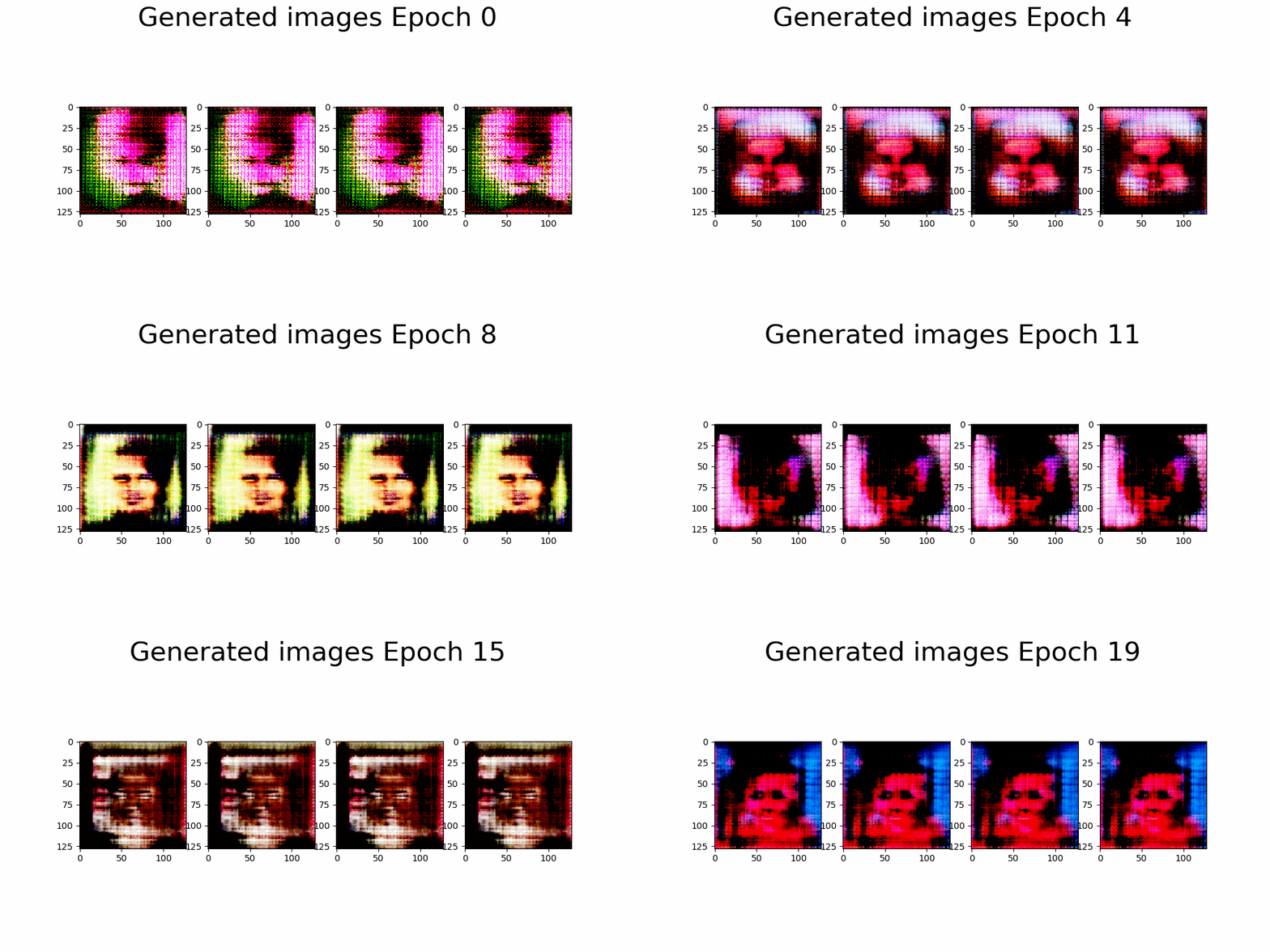
| Trainning size = 10.000 Trainning Epochs = 20 Batch Size = 16 |
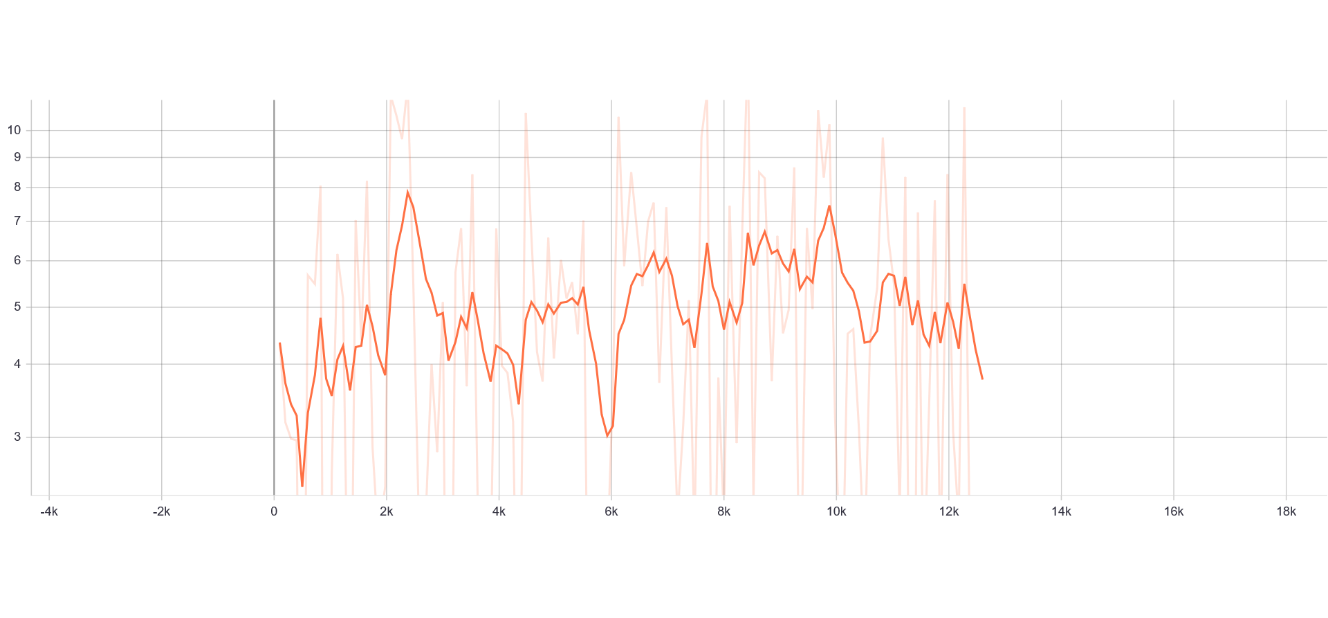
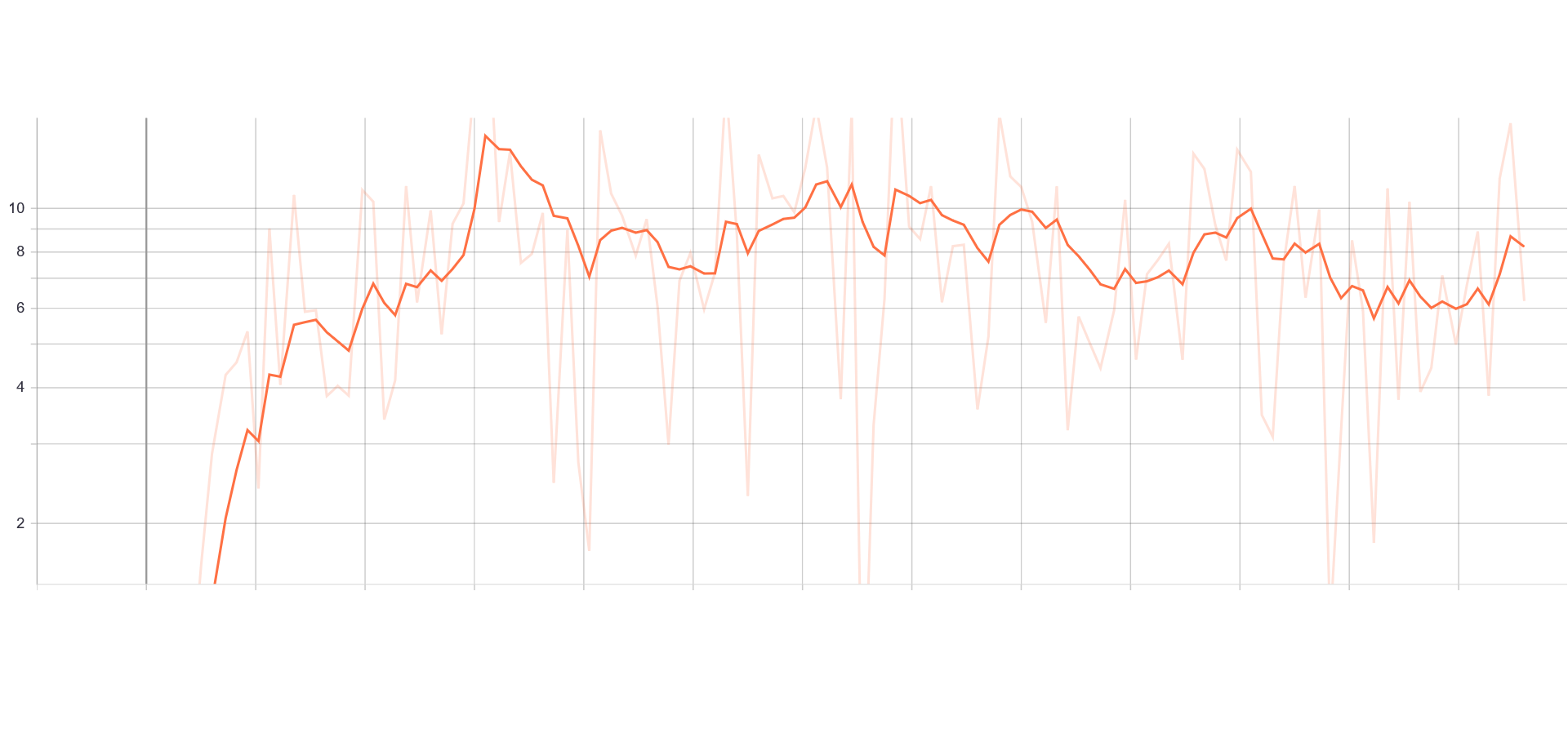
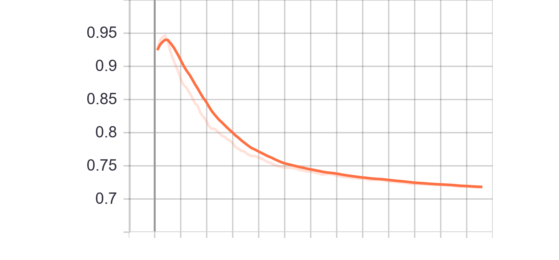
Loss and Accuracy Charts:
 |
 |
|---|---|
| Generator Loss | Discriminator Loss |
 |
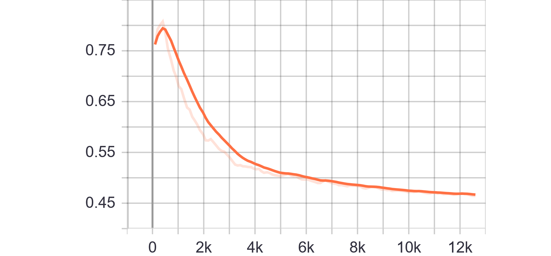 |
| Fake accuracy | Real accuracy |
| Results GIF |
|---|
 |
Change from previous models:
- Removed restriction on D update
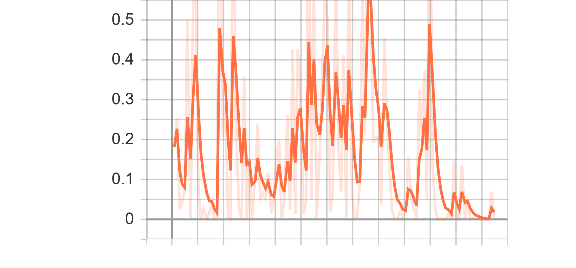
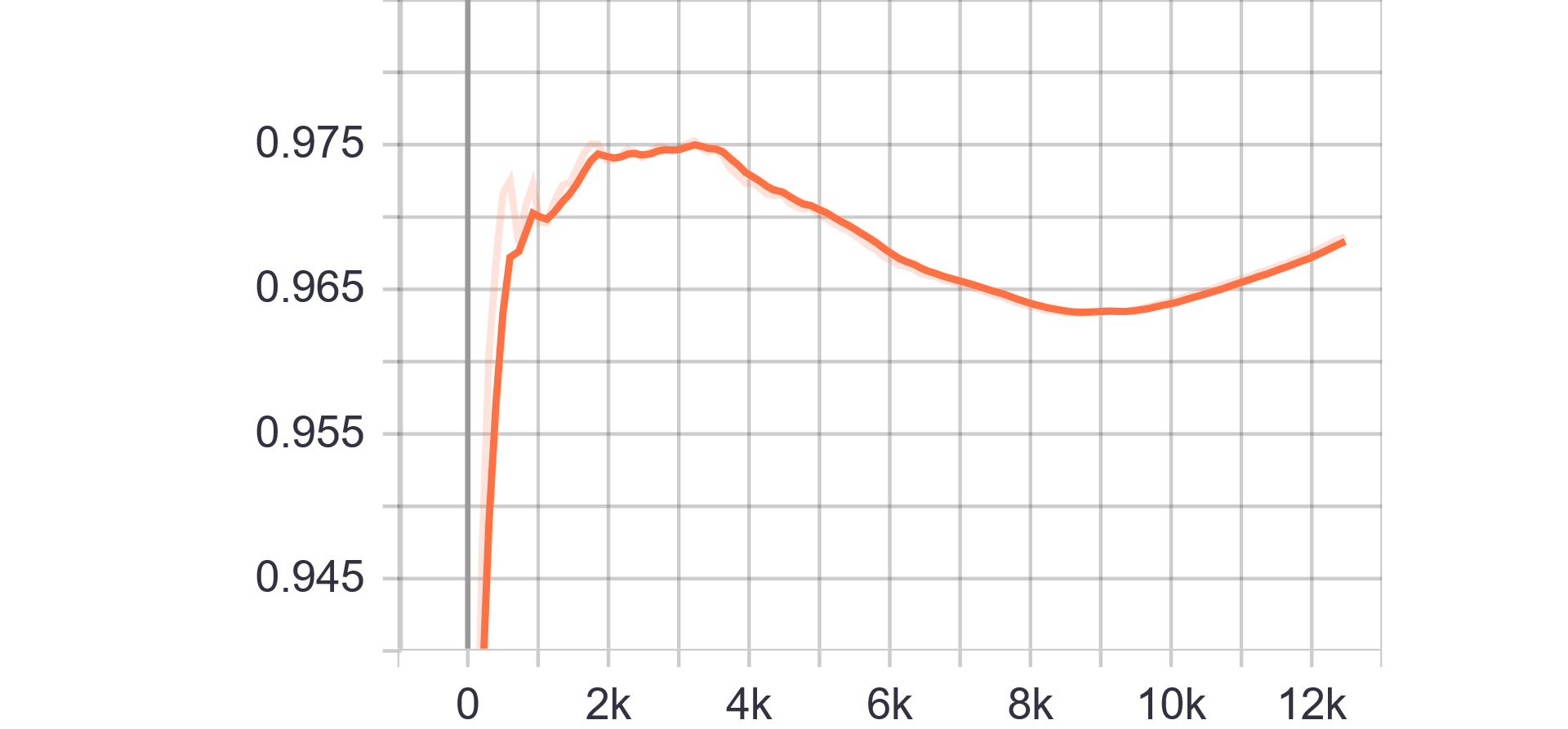
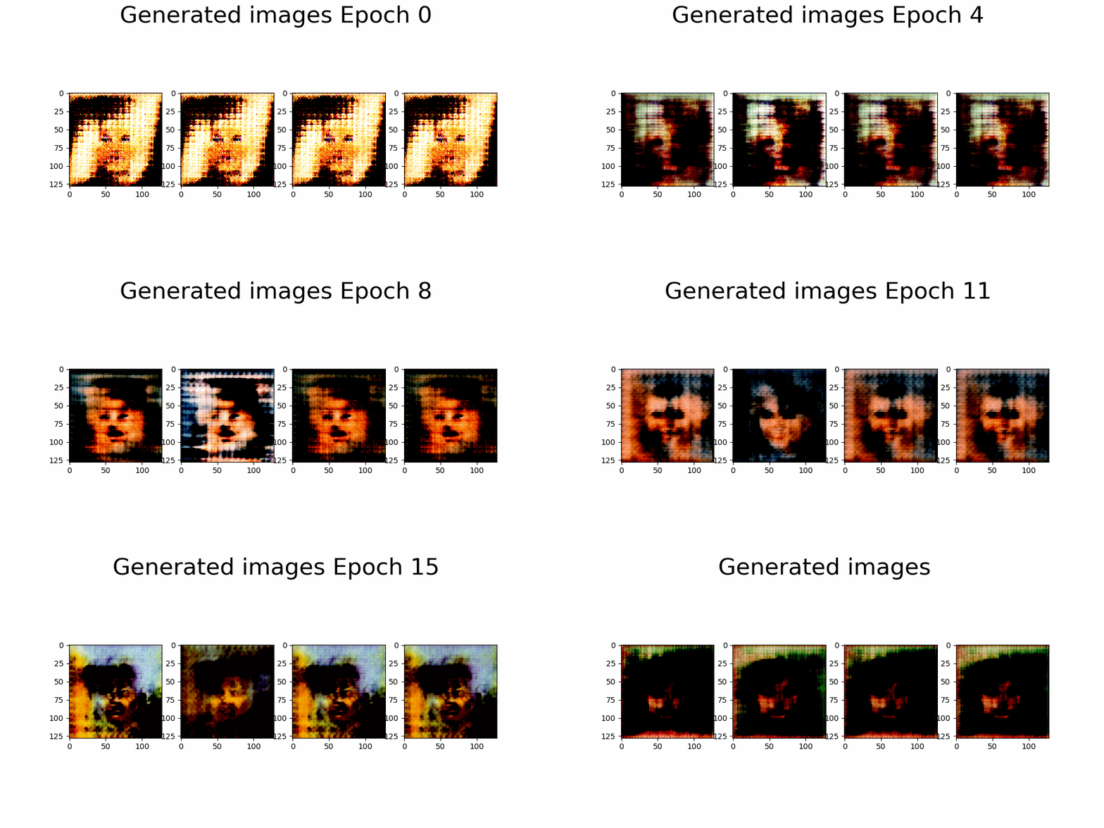
| Hyperparameters | Observations |
|---|---|
| Trainning size = 10.000 Trainning Epochs = 20 Batch Size = 16 |
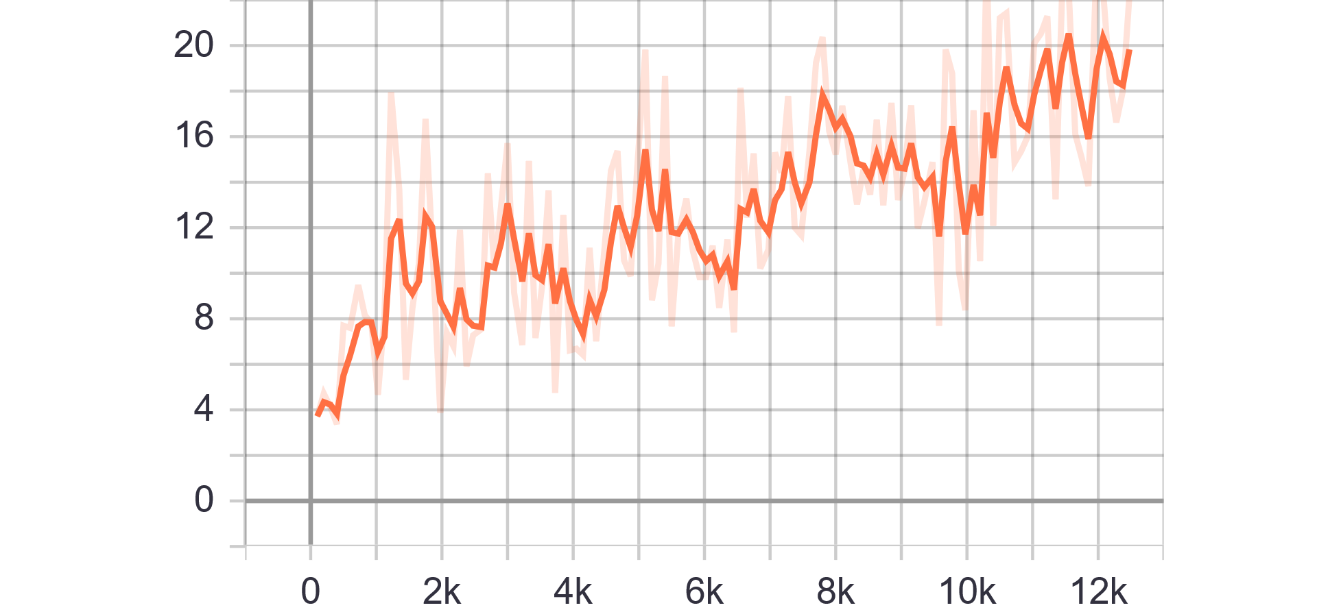
Loss and Accuracy Charts:
 |
 |
|---|---|
| Generator Loss | Discriminator Loss |
 |
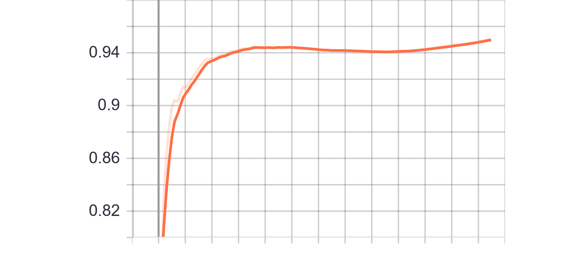 |
| Fake accuracy | Real accuracy |
| Results GIF |
|---|
 |
Change from previous models:
- Added label smoothing (0 -> {0-0.1} and 1 -> {0.9-1})
- Added label flipping on 5% of labels
| Hyperparameters | Observations |
|---|---|
| Trainning size = 10.000 Trainning Epochs = 20 Batch Size = 16 |
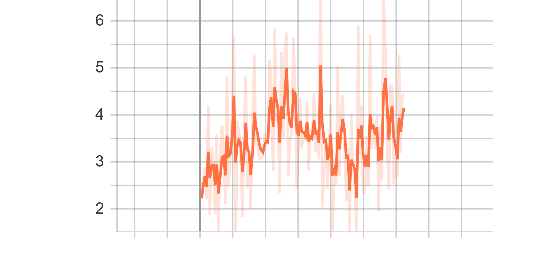
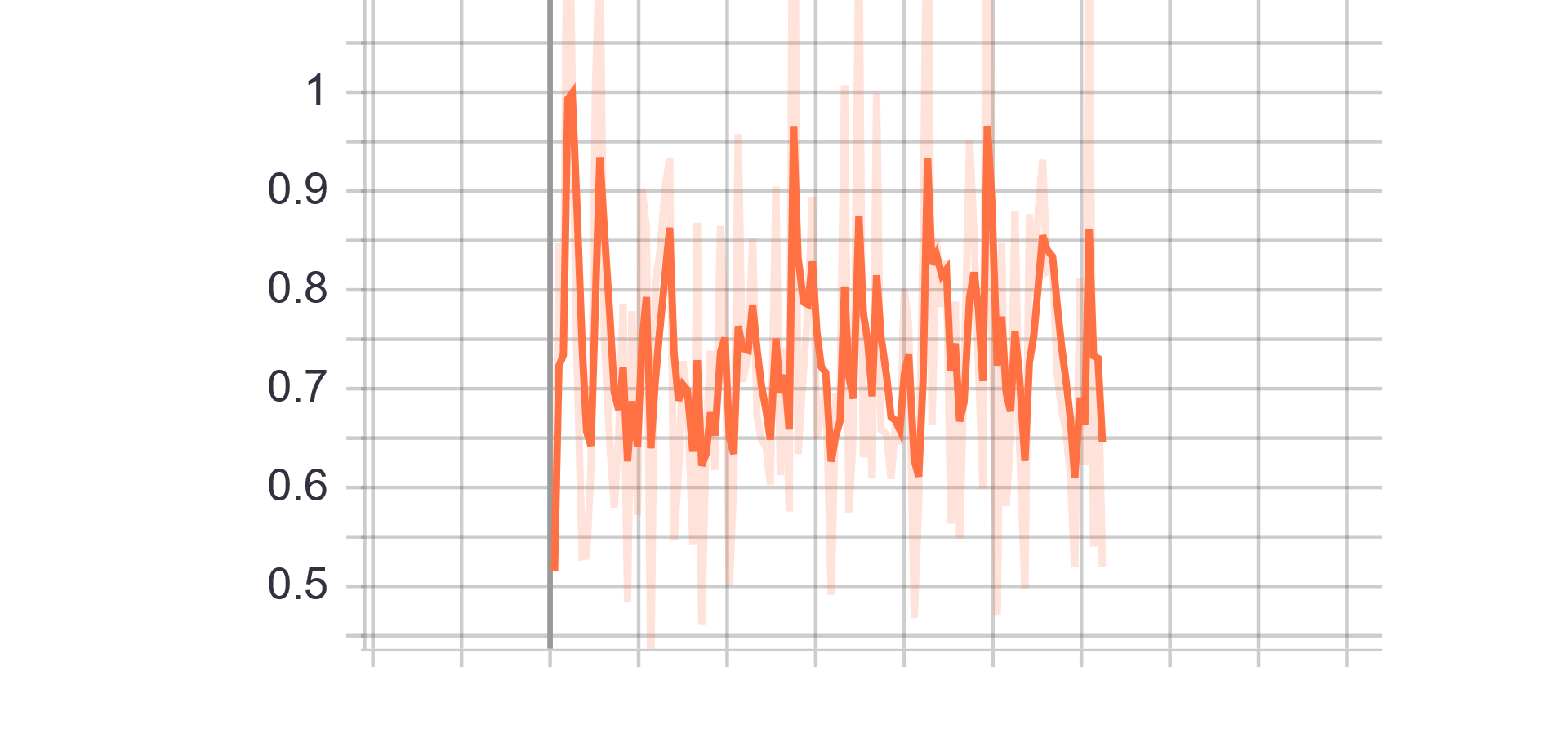
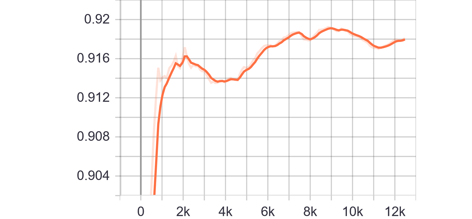
Loss and Accuracy Charts:
 |
 |
|---|---|
| Generator Loss | Discriminator Loss |
 |
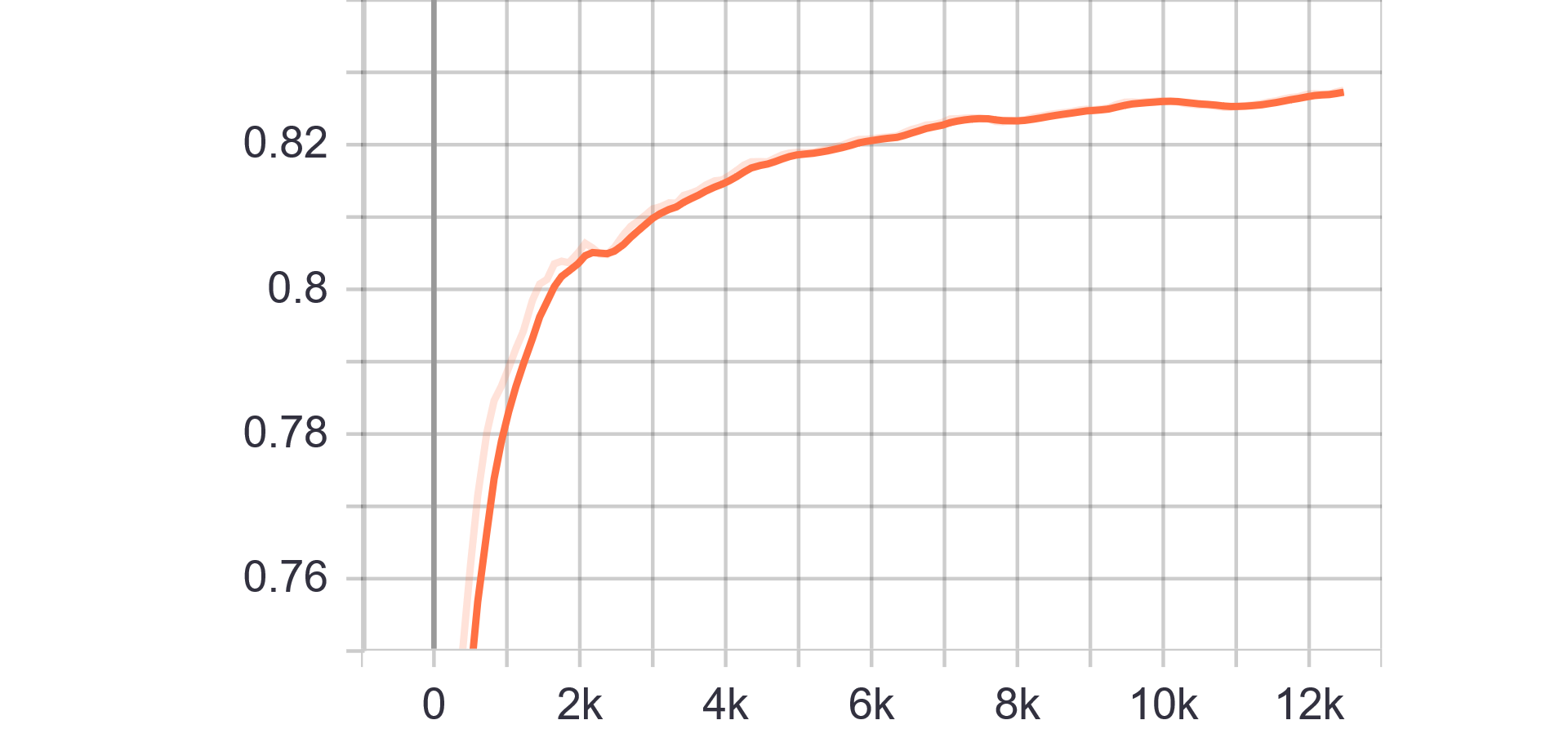 |
| Fake accuracy | Real accuracy |
| Results GIF |
|---|
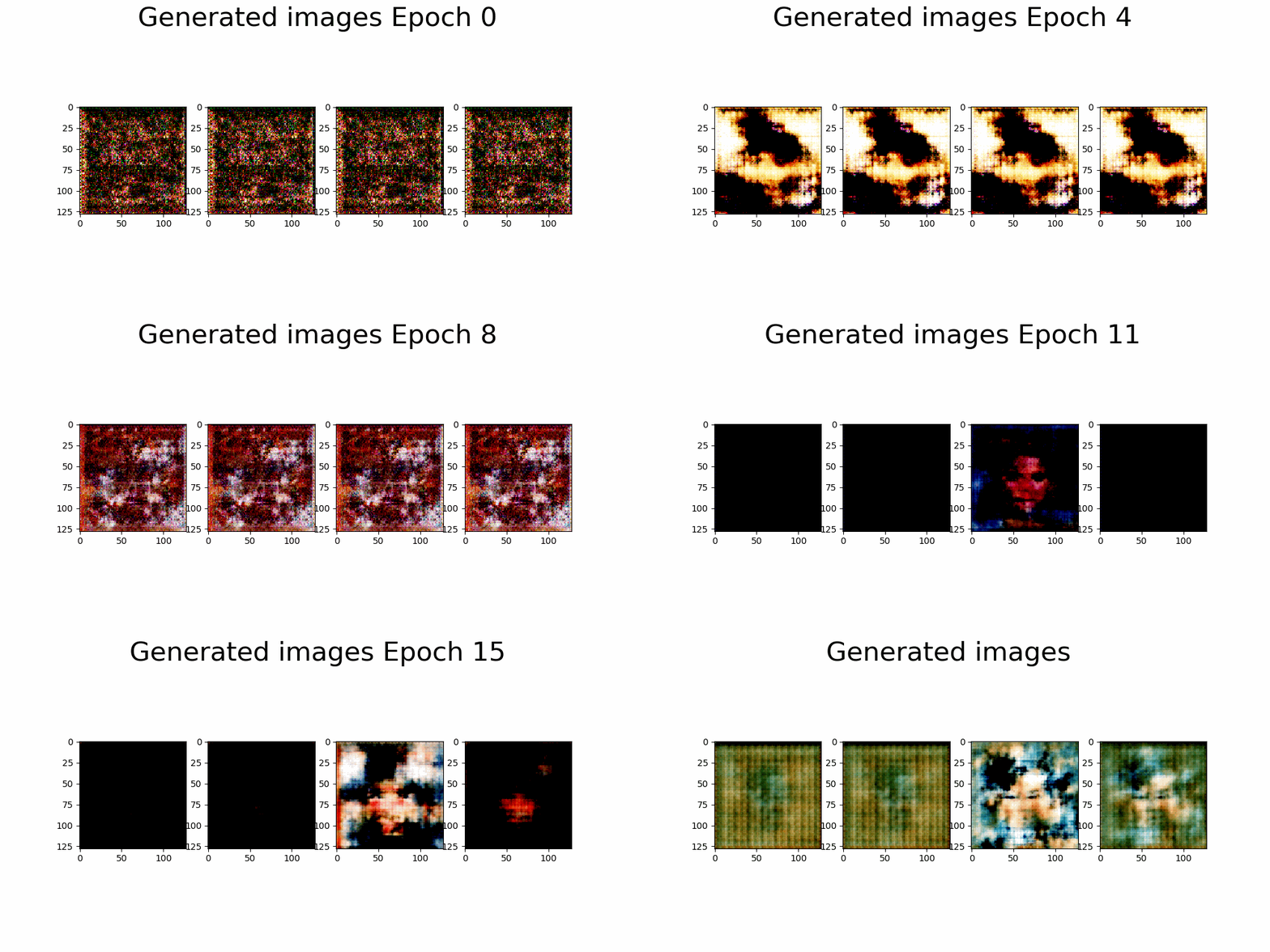 |
Change from previous models:
- Change model architecture.
- Remove BatchNorm layers
- Remove Label Smoothing and Label flip
| Hyperparameters | Observations |
|---|---|
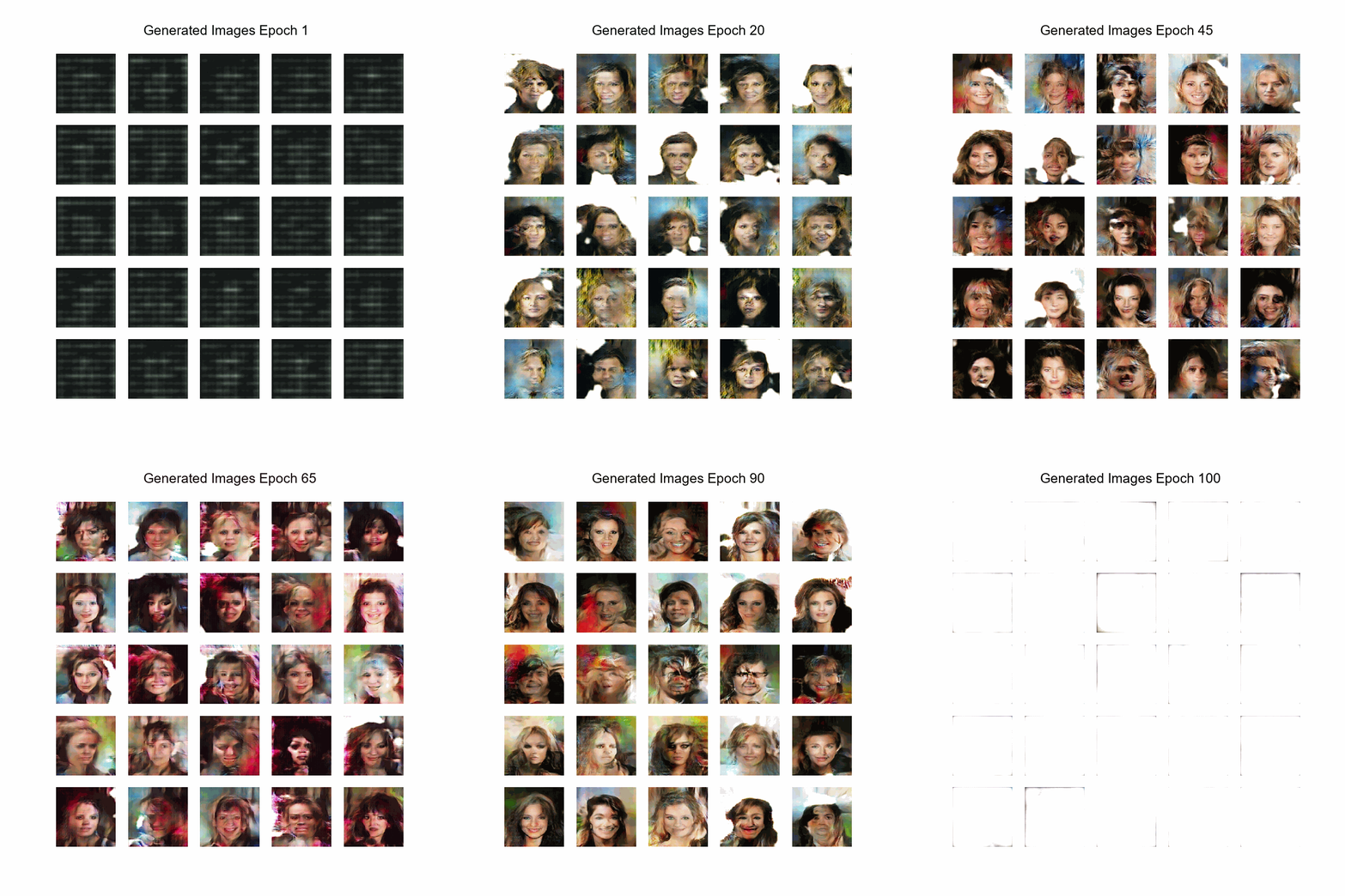
| Trainning size = 10.000 Trainning Epochs = 100 Batch Size = 200 |
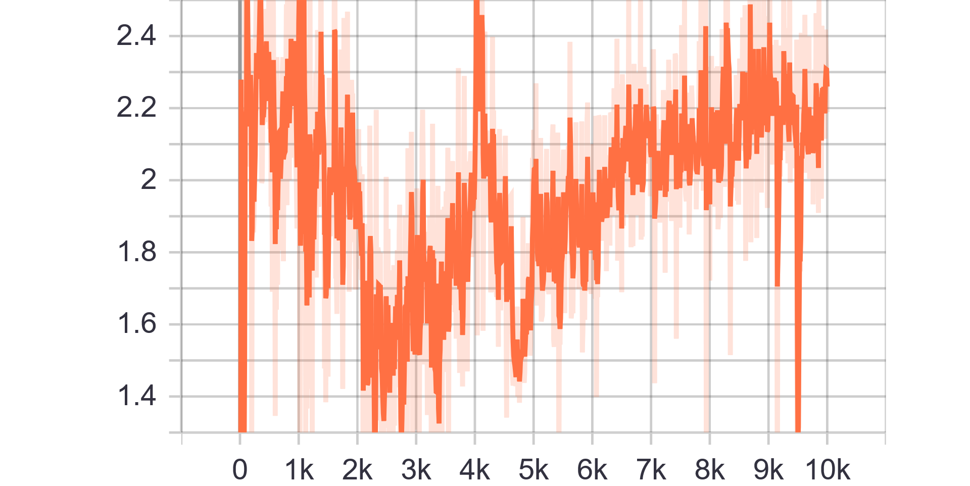
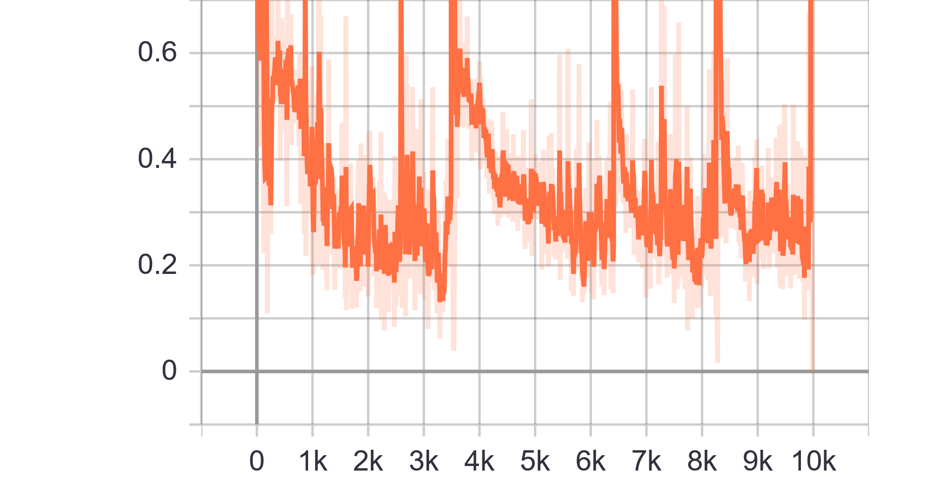
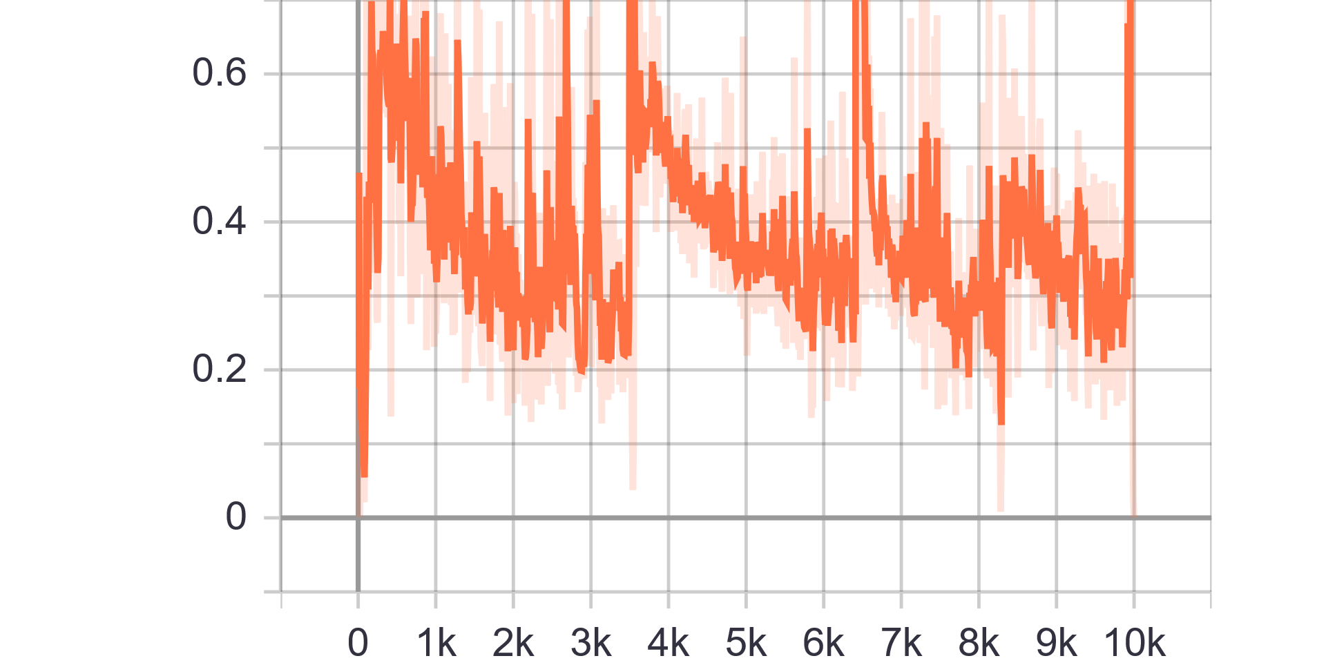
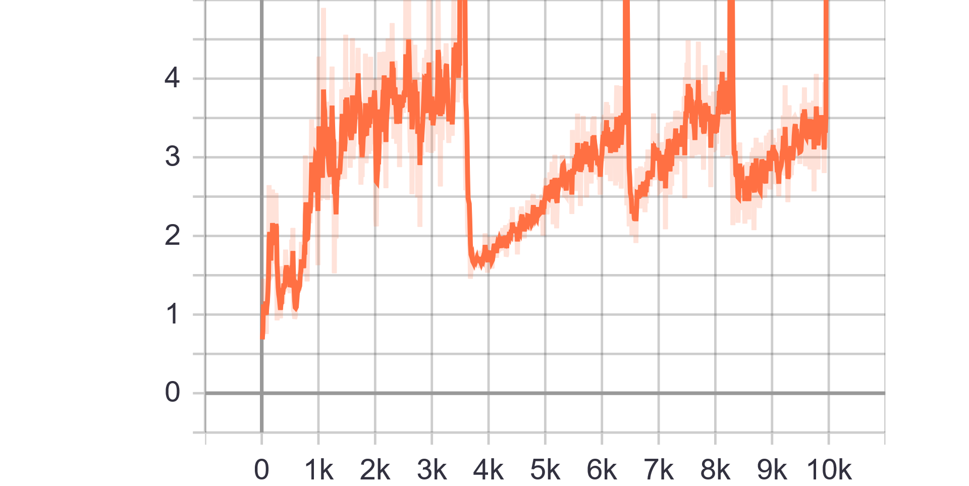
Loss Charts:
 |
 |
|---|---|
| Discriminator Loss Fake | Discriminator Loss Real |
 |
|
| Generator Loss |
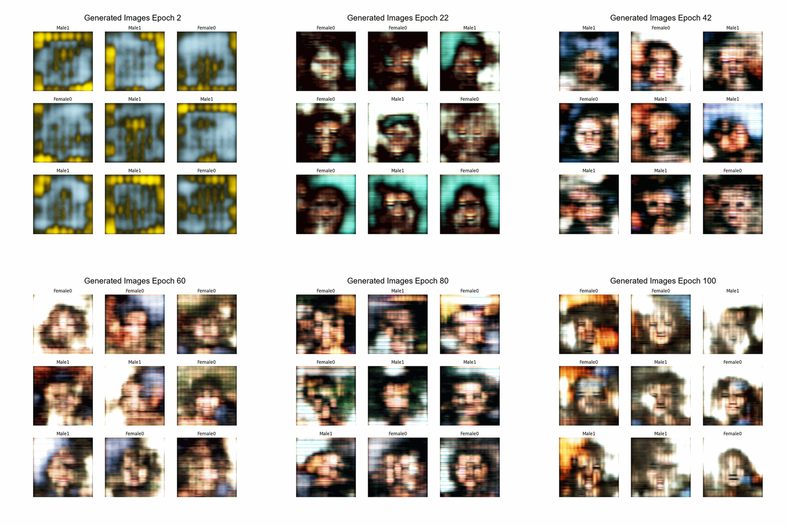
| Results GIF |
|---|
 |
Change from previous models:
- Only male images
- Added label smoothing (0 -> {0-0.1} and 1 -> {0.9-1})
- Added label flipping on 5% of labels
| Hyperparameters | Observations |
|---|---|
| Trainning size = 22.000 Trainning Epochs = 100 Batch Size = 200 |
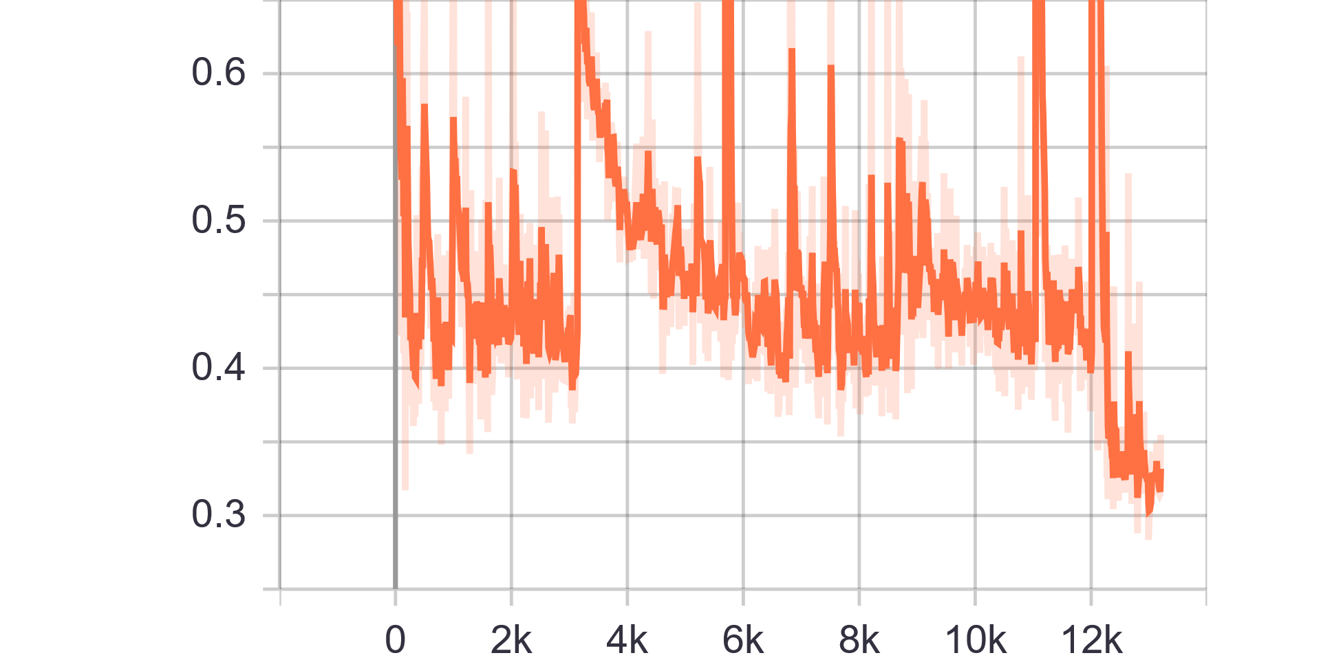
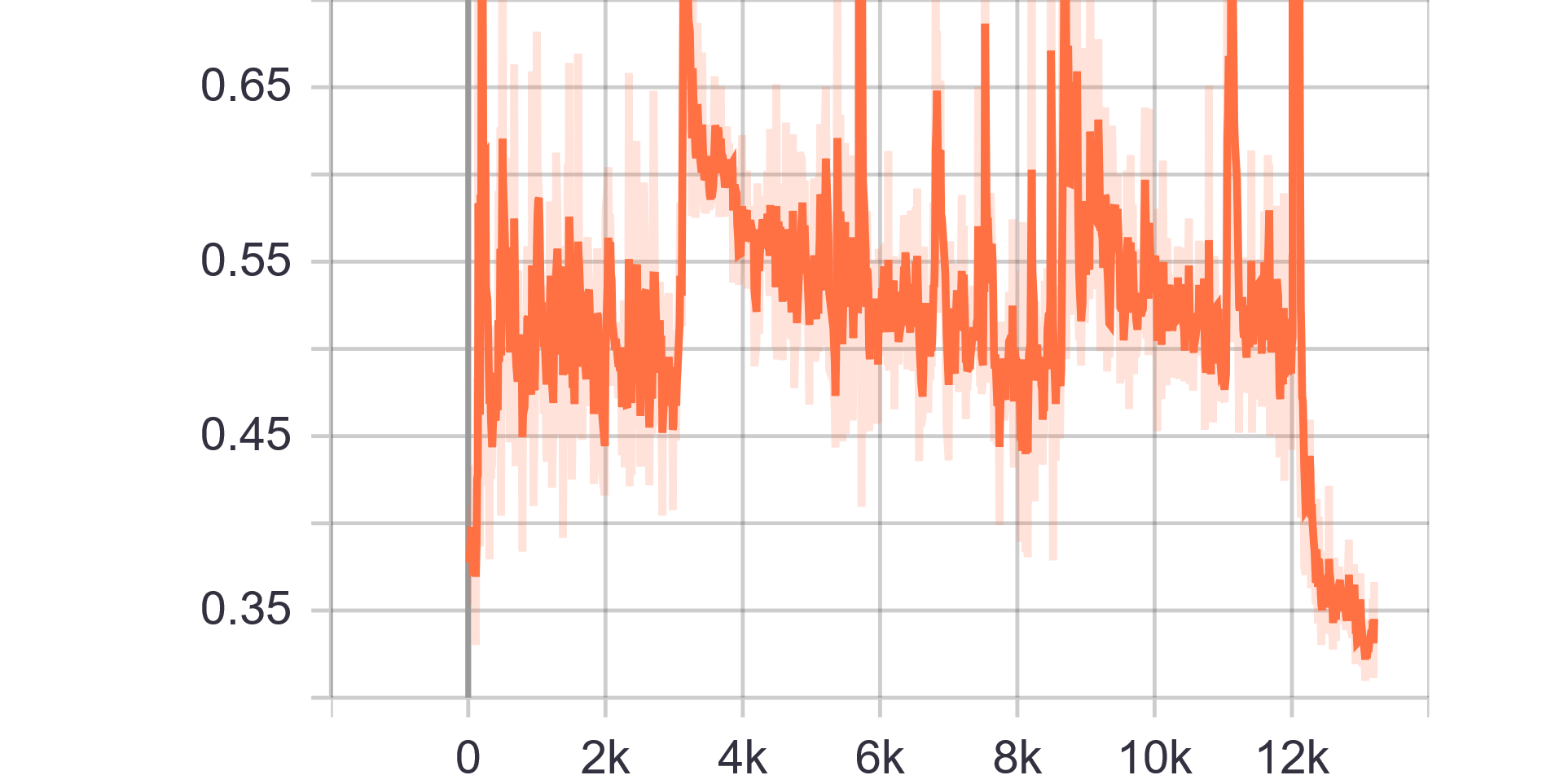
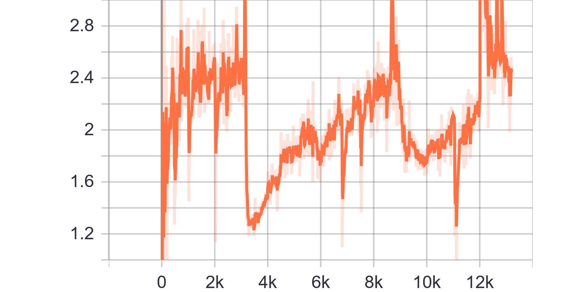
Loss Charts:
 |
 |
|---|---|
| Discriminator Loss Fake | Discriminator Loss Real |
 |
|
| Generator Loss |
| Results GIF |
|---|
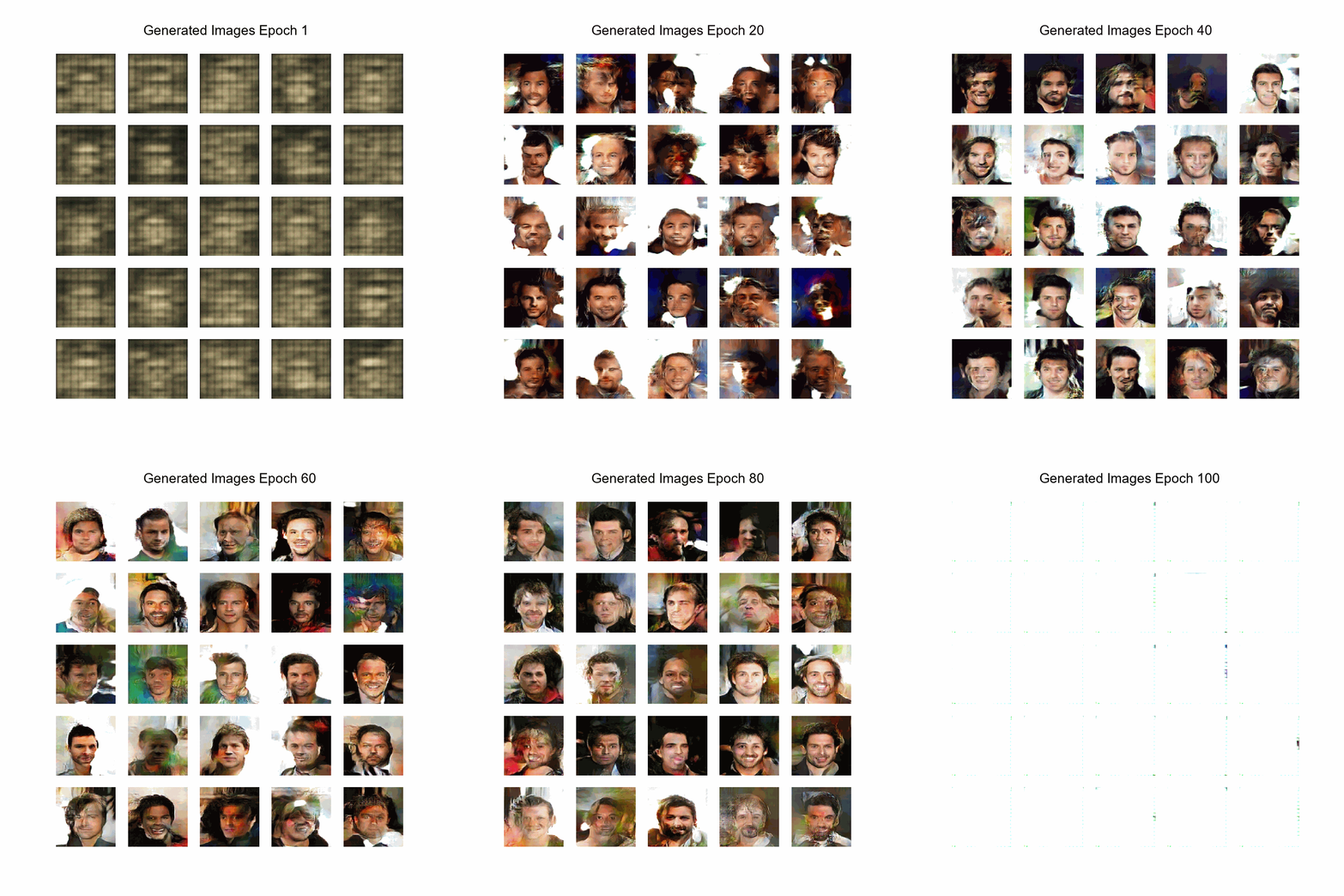 |
Change from previous models:
- Using male and female images at 50%
- Introduced training ratio G:D, set to 1:3 (traing D 3 times more than G)
| Hyperparameters | Observations |
|---|---|
| Trainning size = 10.000 Trainning Epochs = 100 Batch Size = 100 |
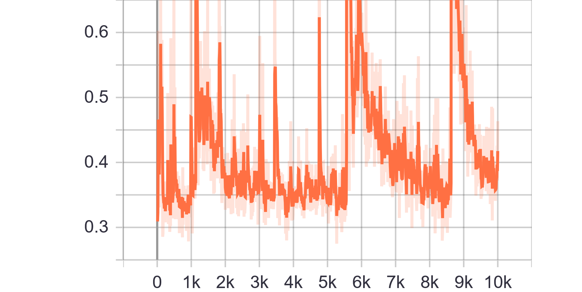
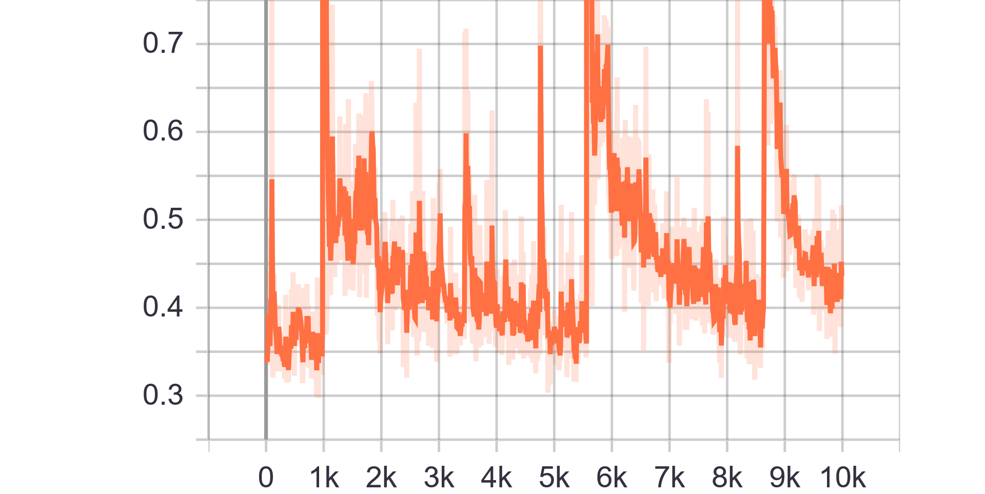
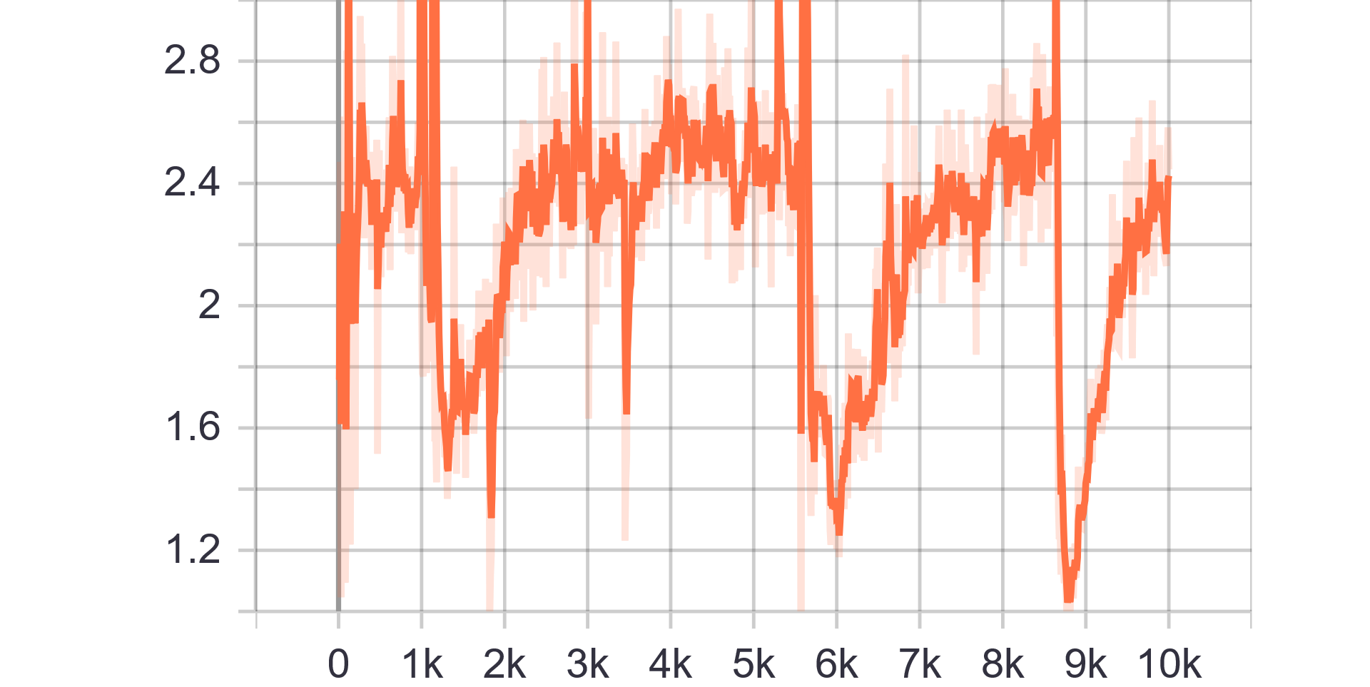
Loss Charts:
 |
 |
|---|---|
| Discriminator Loss Fake | Discriminator Loss Real |
 |
|
| Generator Loss |
| Results GIF |
|---|
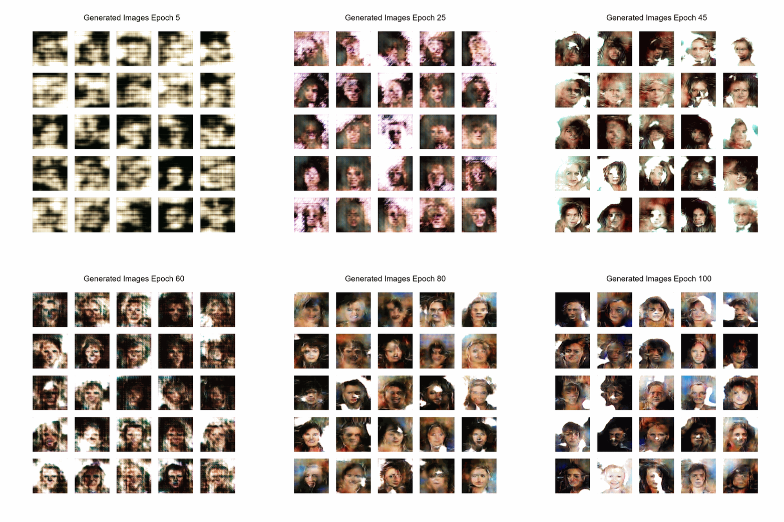 |
Change from previous models:
- Chenge architecture to introduce conditioning GAN
- Only 1 feature allowed for conditioning
- Ratio G:D, set to 1:1
| Hyperparameters | Observations |
|---|---|
| Trainning size = 10.000 Trainning Epochs = 100 Batch Size = 100 |
Loss Charts:
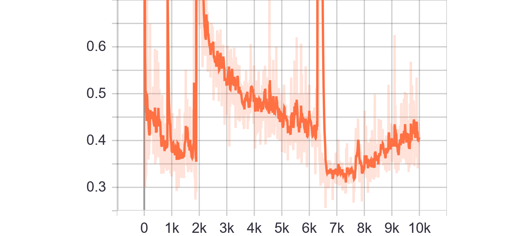 |
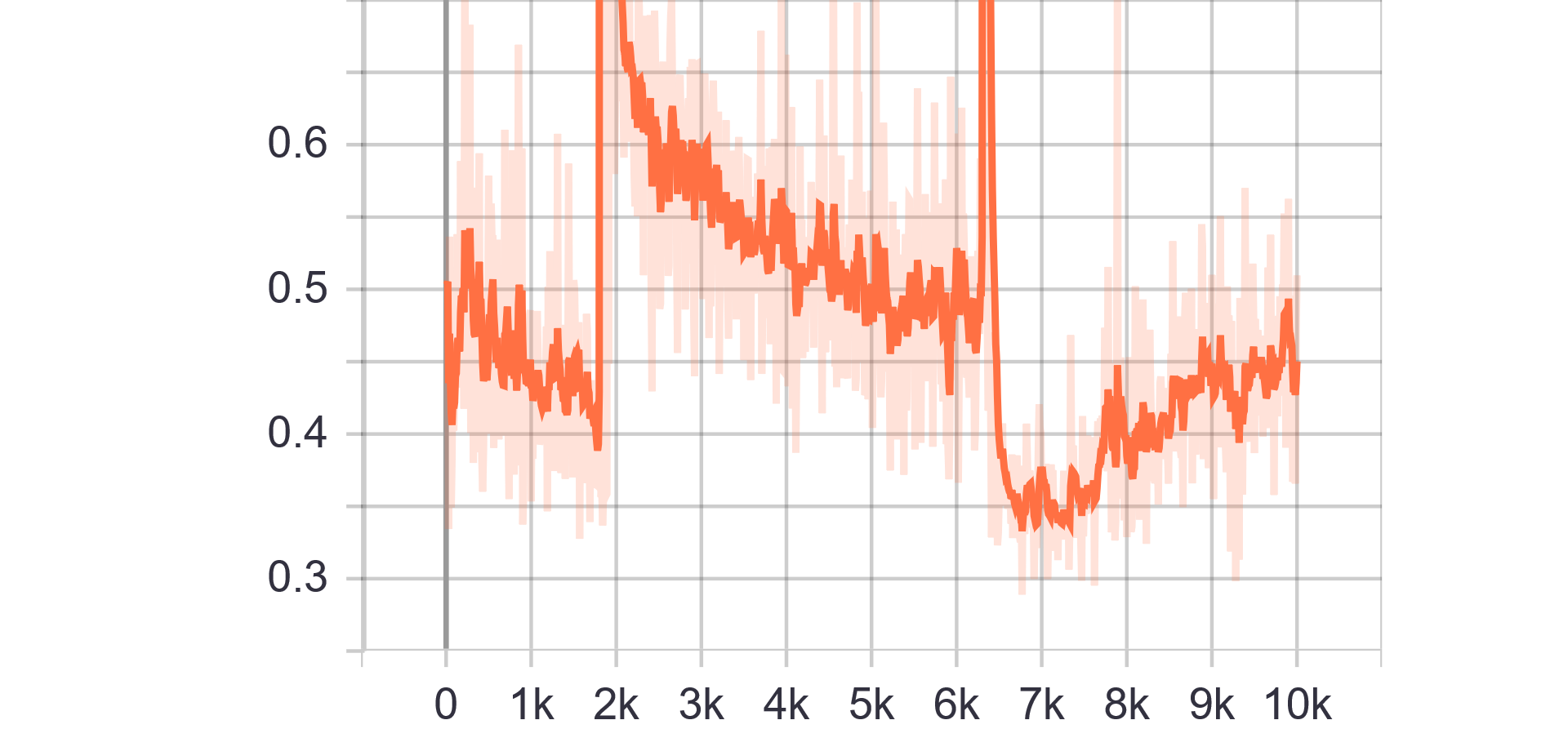 |
|---|---|
| Discriminator Loss Fake | Discriminator Loss Real |
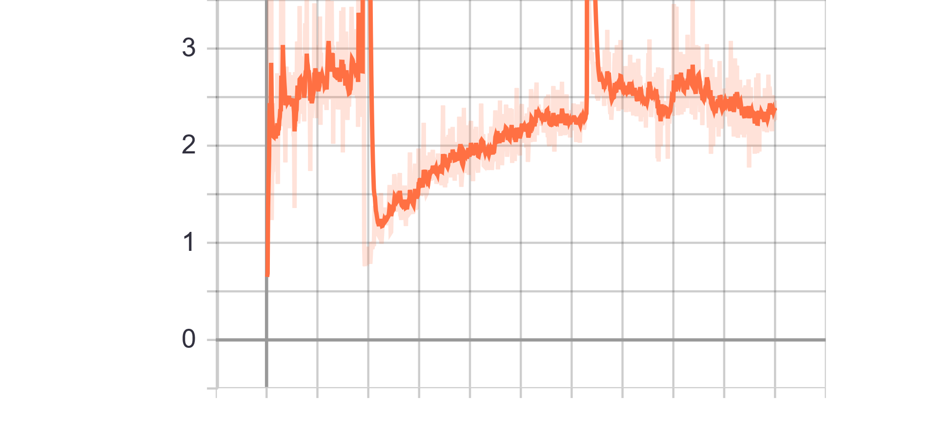 |
|
| Generator Loss |
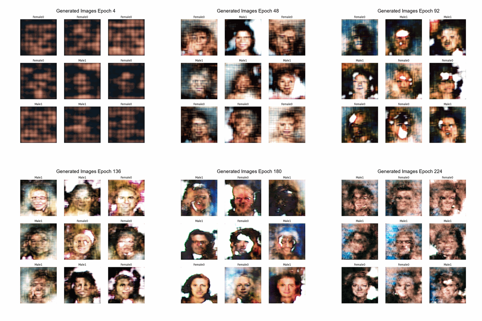
| Results GIF |
|---|
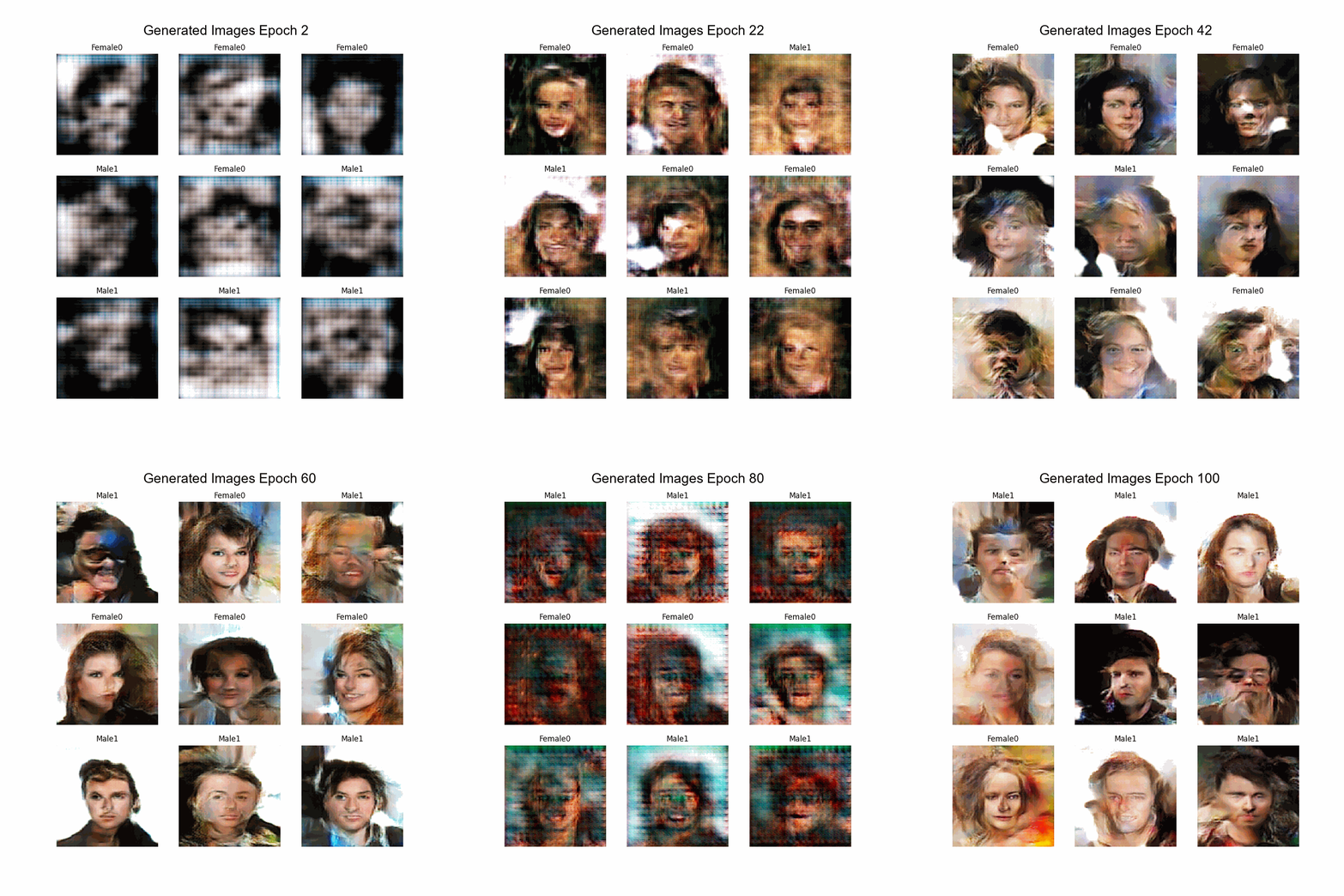 |
Change from previous models:
- Introduced training ratio G:D, set to 1:3 (traing D 3 times more than G)
| Hyperparameters | Observations |
|---|---|
| Trainning size = 10.000 Trainning Epochs = 100 Batch Size = 100 |
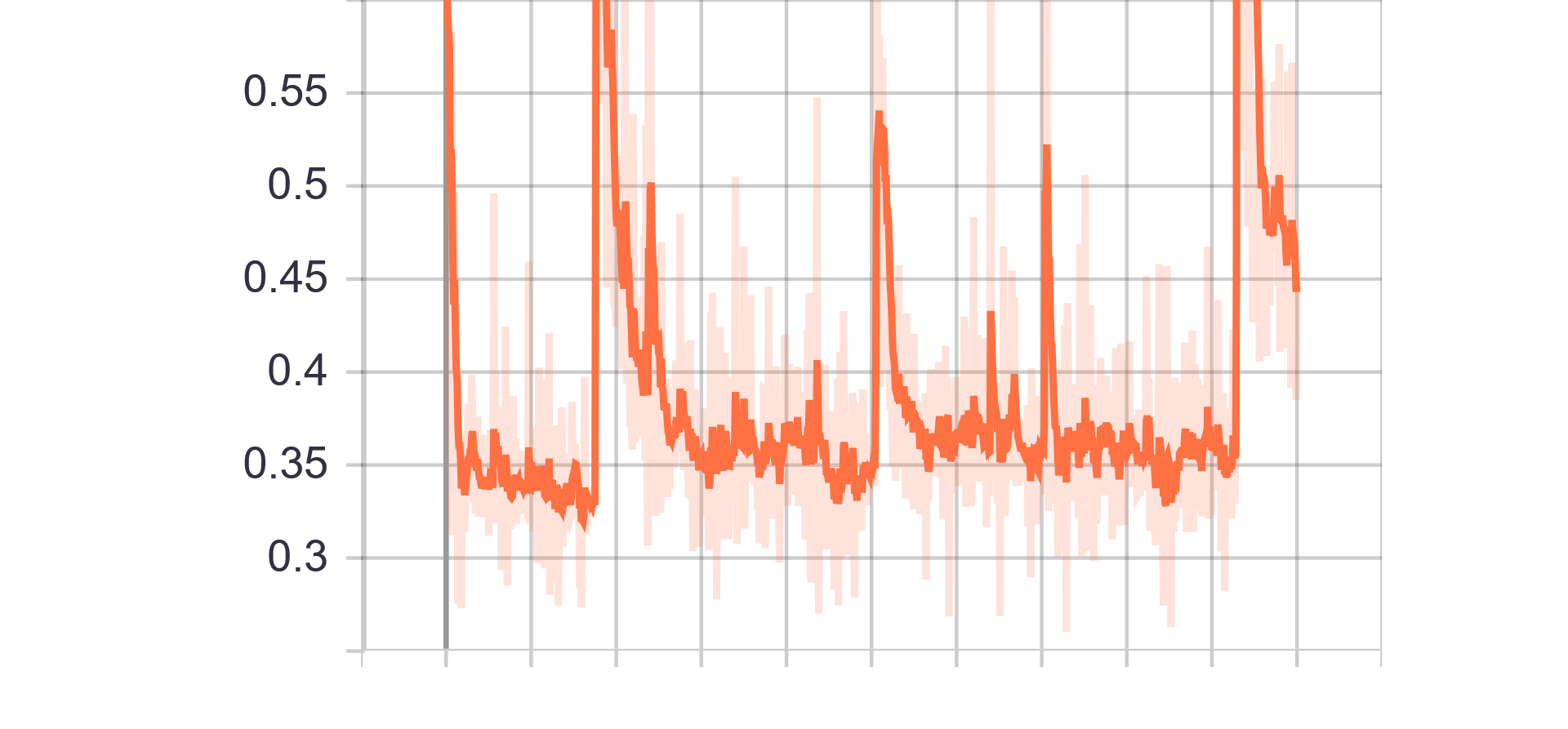
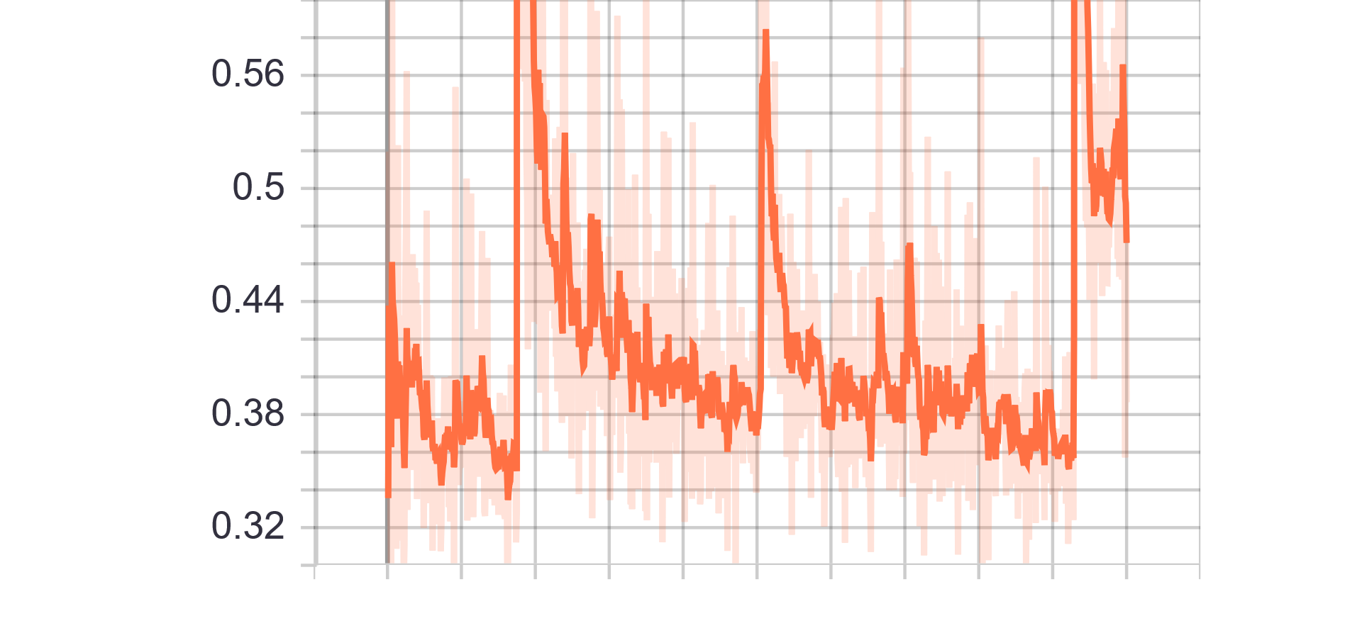
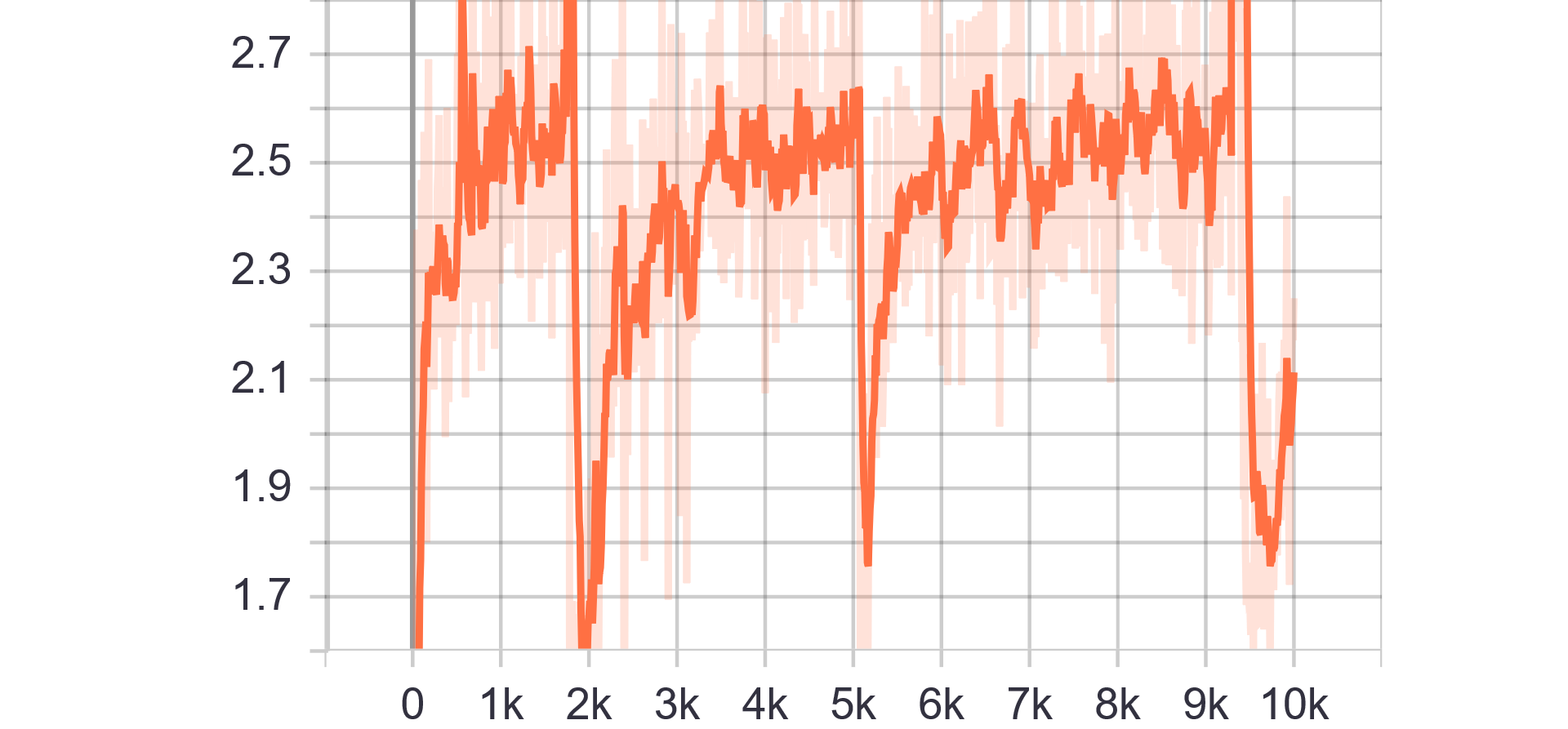
Loss Charts:
 |
 |
|---|---|
| Discriminator Loss Fake | Discriminator Loss Real |
 |
|
| Generator Loss |
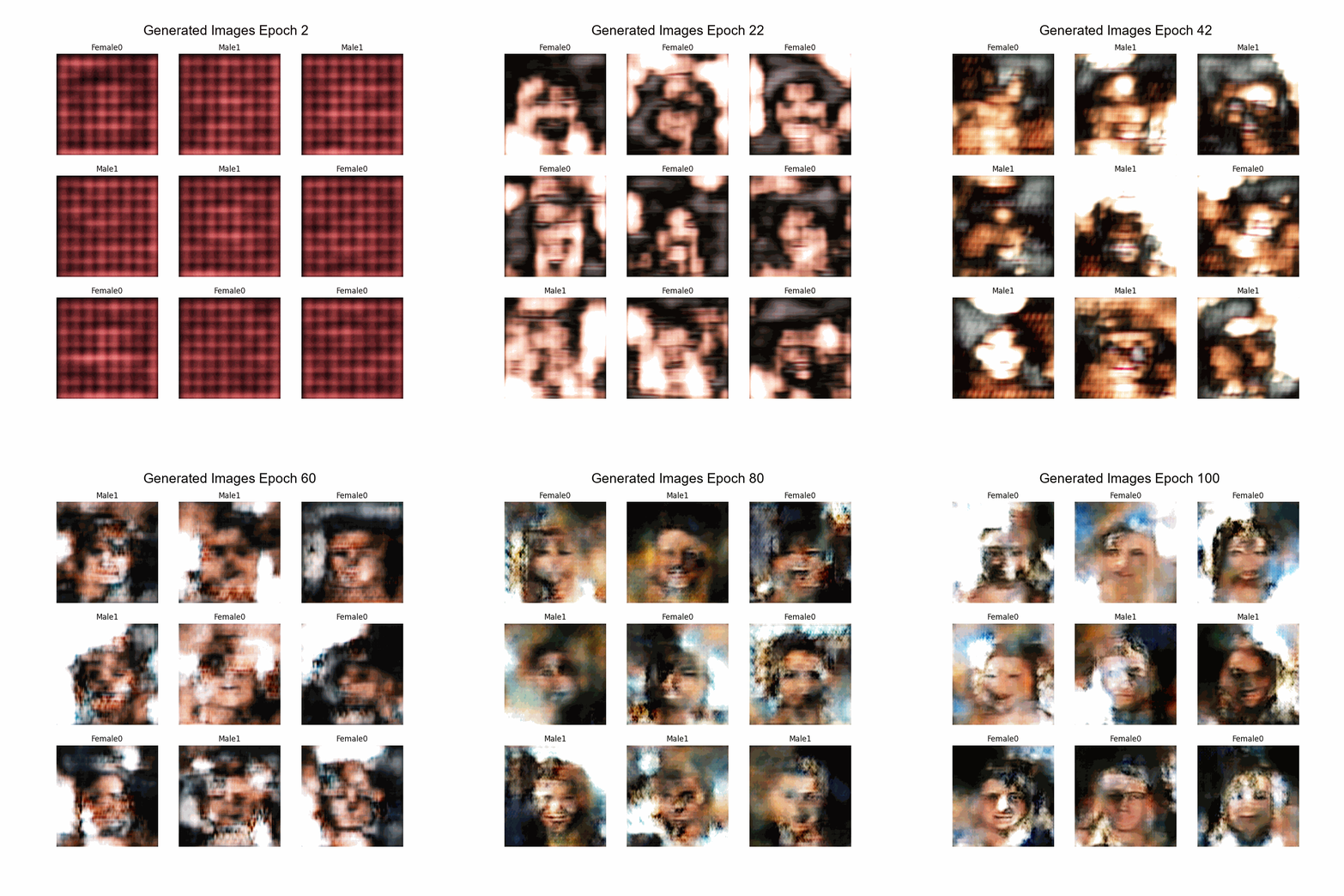
| Results GIF |
|---|
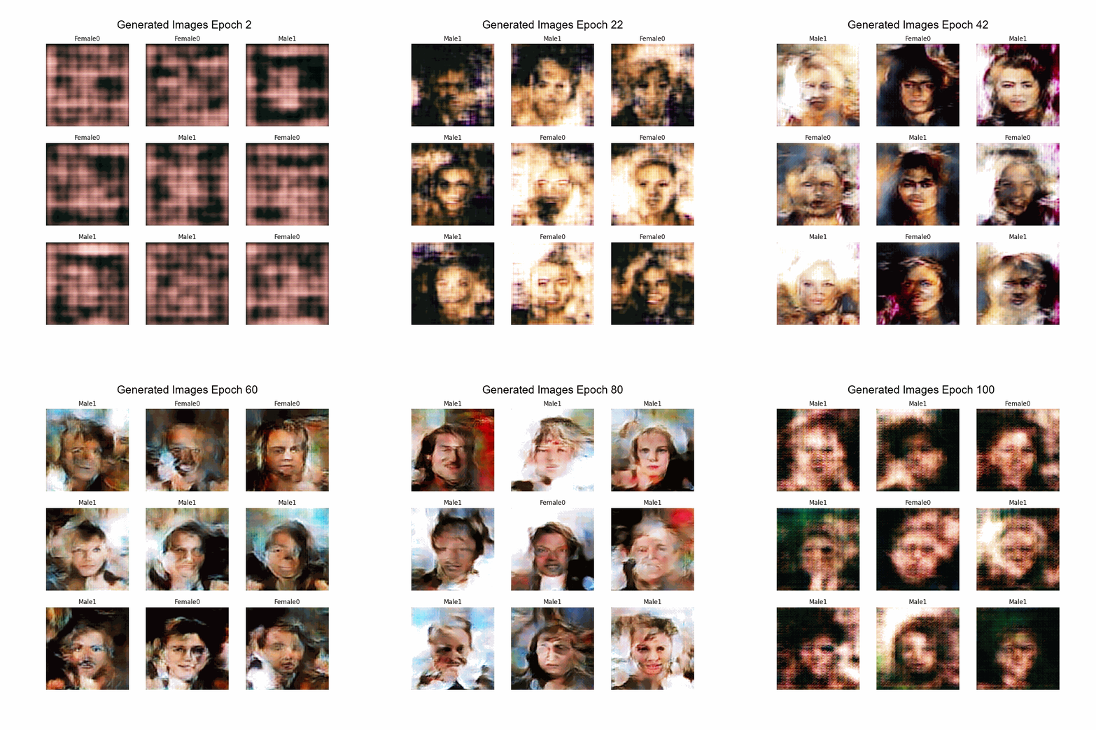 |
Using Experiment 11 as base:
- Introduced Spectral Normalization
- Different ratios of times trained Generator and Discriminator used.
| Hyperparameters | Observations |
|---|---|
| Trainning size = 10.000 Trainning Epochs = 100\220\100 Batch Size = 100 Ratio of training G:D = 1:1\1:3\1:5 |
* The final images are not good enough as the ones in the previous experiments. * The Spectral Normalization gives stability and prevents the white background images. * To improve results another experiment should be done using Attention and Spectral Normalization which would give better results. |
Loss Charts:
Using Experiment 11 as base:
- Implementation of Multi-labeling
- Labels:
- Bald
- Glasses
- Beard
| Hyperparameters | Observations |
|---|---|
| Trainning size = 9000 Trainning Epochs = 100 Batch Size = 100 |
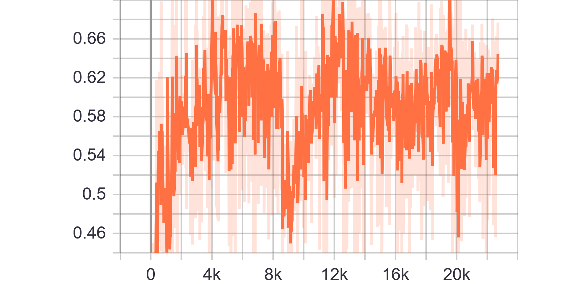
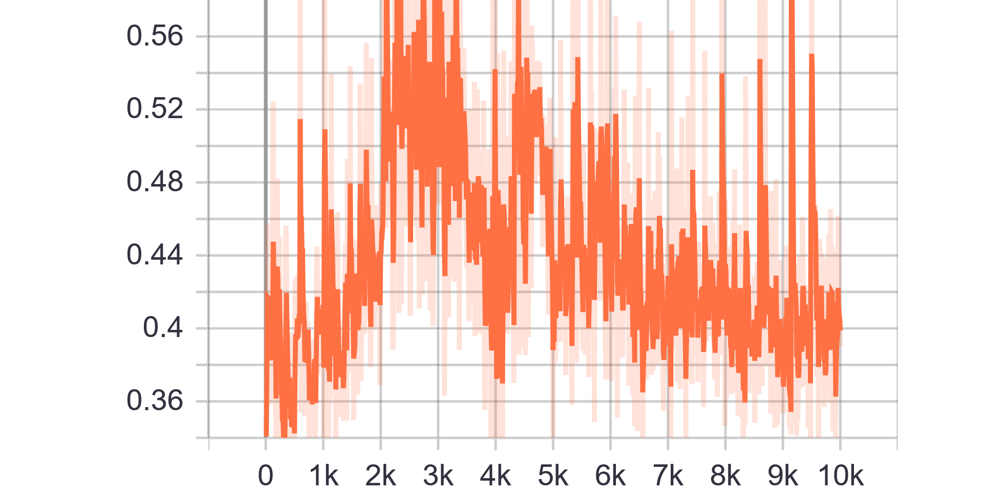
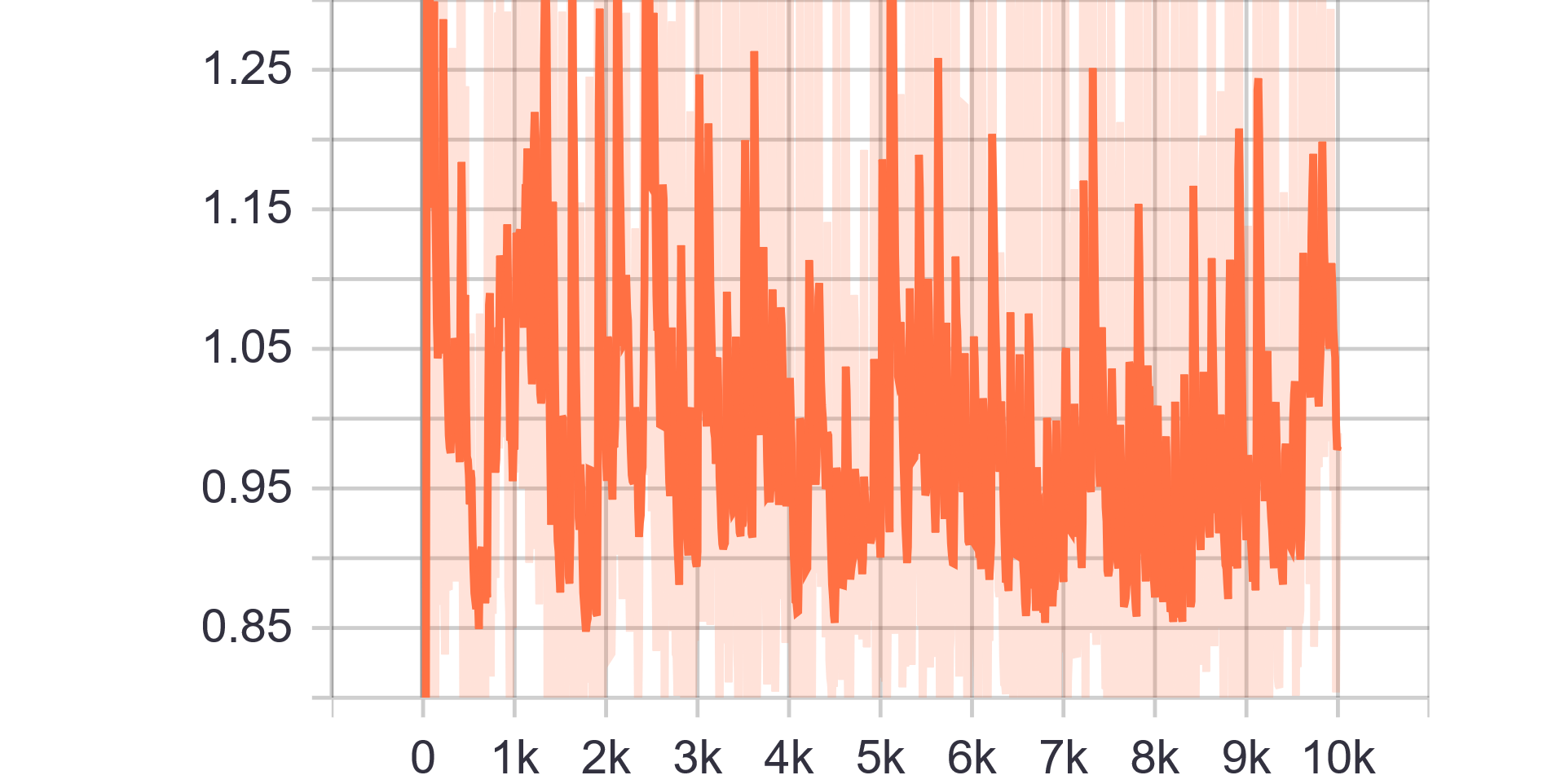
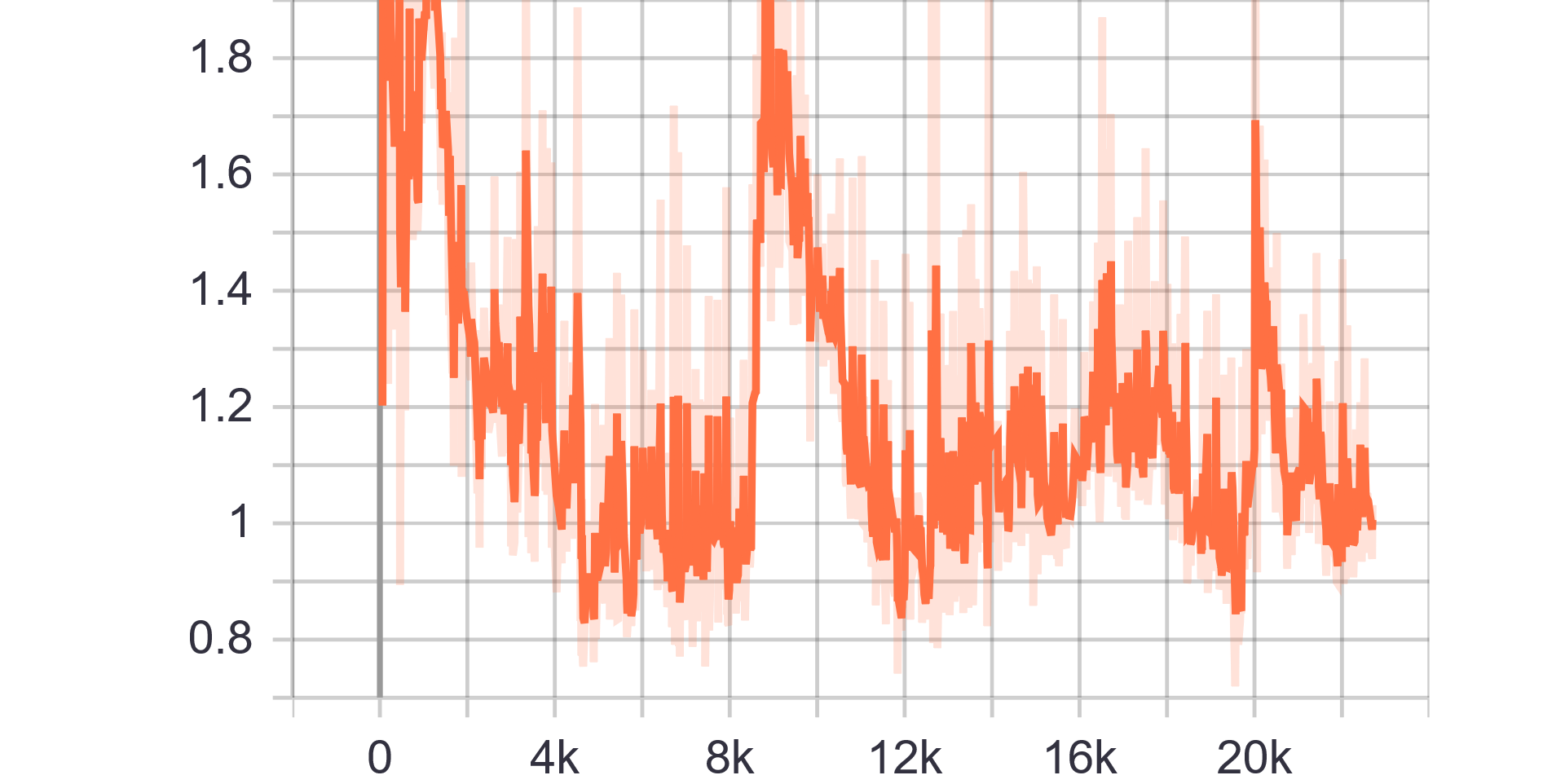
Loss Charts:
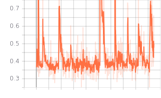 |
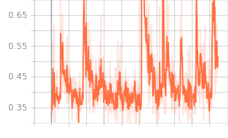 |
|---|---|
| Discriminator Loss Fake | Discriminator Loss Real |
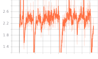 |
|
| Generator Loss |
- Albert Nieto
- Luis Tuzón
- Jordi Sans
- Mauro Álvarez


