The objective of this project is to forecast wildfires in Australia for February 2021. The estimated fire area represents the summation of fire activity in a 1km by 1km region. The Australian 7 regions are:
- NSW = New South Wales
- NT = Northern Territory
- QL = Queensland
- SA = Southern Australia
- TA = Tasmania
- VI = Victoria
- WA = Western Australia
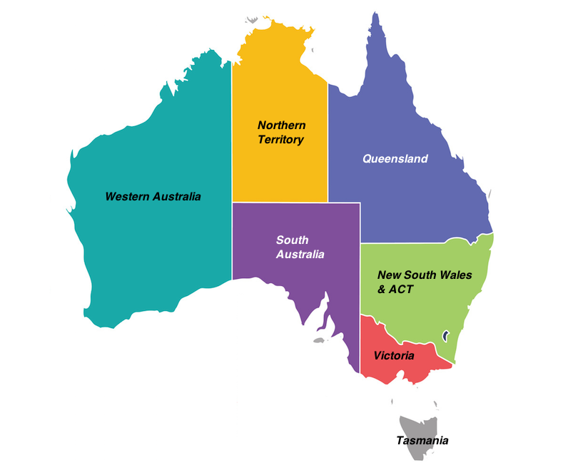
credit: https://www.touropia.com/regions-in-australia-map/
The original zip datafile can be retrieved from the code challenge git page; provided here.
The zipped data file includes the following:
Nov_10
└───Historical_Wildfires.csv
│   └─── :: Contains data on fire activites in Australia from 2005.
└───HistoricalWeather.csv
│   └─── :: Contains daily aggregates of weather including Precipitation
│        :: Humidty, Soil water content, Solar Radiation, Temperature
│        :: and Wind Speed.
└───HistoricalWeatherForecasts.csv
│   └─── :: Contains forecasted values for weather in 5, 10 or 15 lead times.
└───LandClass.csv
│   └─── :: Contains terrain properties of the 7 regions pulled on 2015.
└───VegetationIndex.csv
    └─── :: Contains monthly vegetation values(min, max, mean, variance)
         :: for each region
The Historical_Wildfires dataset is based on the MCD14DL dataset (comprised of MOD14AL1/MYD14AL1, which highlights thermal anomalies with a pixel resolution of 1000 meters). The dataset has daily time intervals ranging from 2005-01-01 to 2020-10-31'. The "estimated fire area" was computed by multiplying the scan and track pixel sizes from the MCD14DL. The areas are then totaled by region daily to return the historical wildfires csv.
The pixels from MODIS represent 1km only directly below the satellite, and the scan and track values are calculated due to increasing resolution as the pixels approach the end of the picture. The scan and track represent the spatial resolution east to west and north to south respective. It's important to note that all pixels do not represent 1km in a spatial area, and the resolution increases as the pixels are further away from the center.
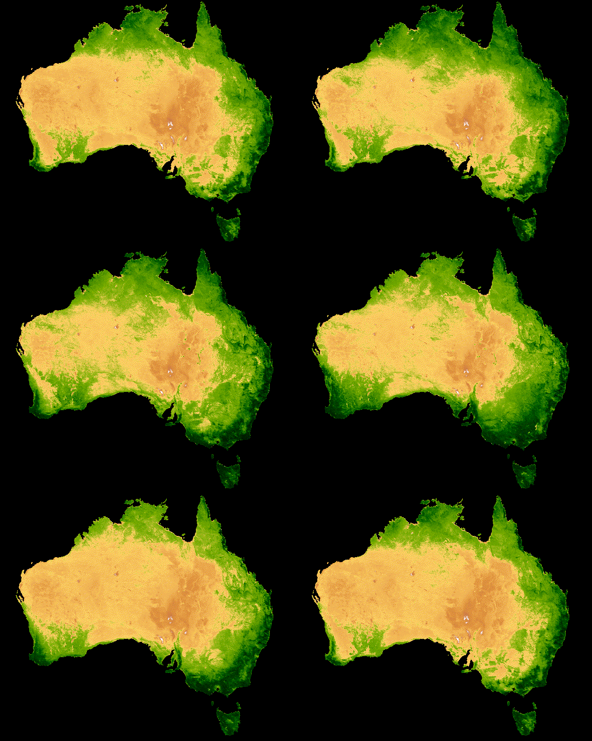
The weather and vegetation data was also aggragagated by mean, min, max, and standard deviation. The following gif represents the NDVI values for Australia in 2020. I included this gif to show how large the original datasets are before compression.
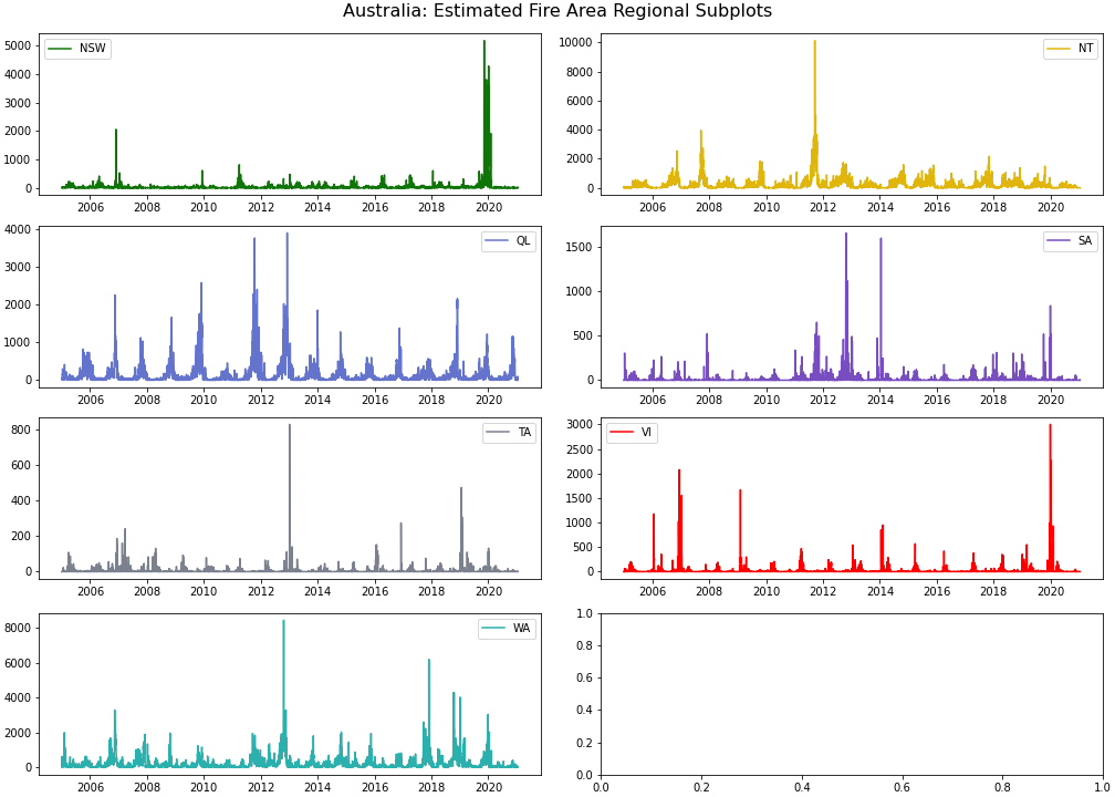
Here I have plotted the daily estimated fire area per region. The land cover area differs for each region, nonetheless, the pattern of daily fire areas are not uniform across all regions.
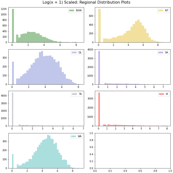
Like most natural disasters, wildfires often come in power-law like distributions and therefore I log transformed for this plot to see the distributions of each region. This can be quickly interpretted that the distributions of fires are not uniform across the 7 regions.
The dependent variable for this project is the estimated fire area per region. The data statistics are aggregated per region and are not granulated to the point where I'll be able to plot the datapoints geographically. The same thing applies to the weather and vegetation statistics. Therefore, we will also assume the variables regarding wildfires, weather, and vegetation to be uniformly distributed per region. (This may not be exactly what we want, and further data collection might be done; please see Further Steps)
We will also assume that natural fires tend to have a life expectancy and don't live perpetually(One tree won't burn until the end of time). However, the real risk is the expansion of fires. For example, although one tree stopped burning, the fire could have expanded to other trees creating a domino effect.
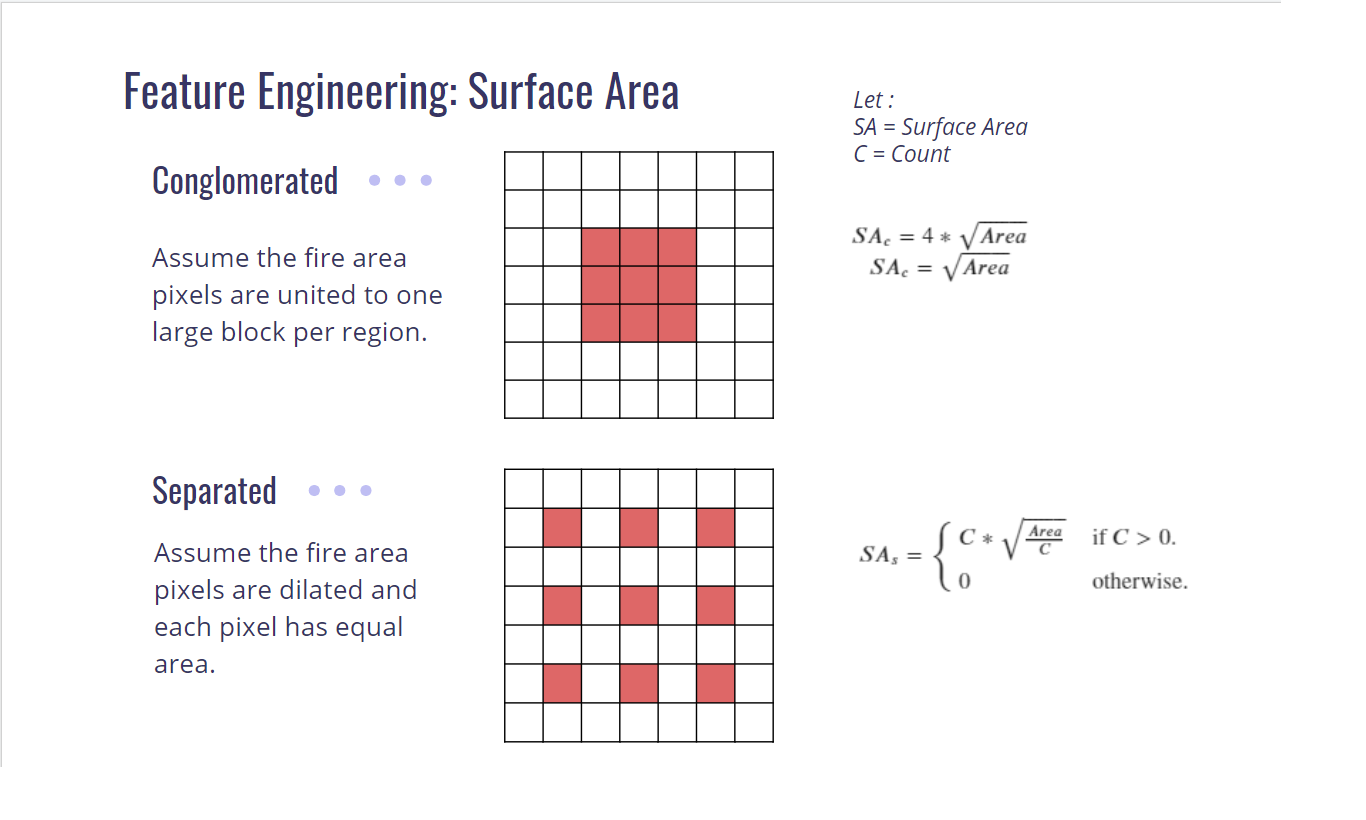
Therefore, a feature that might be interesting would be involving the perimeter of the fire. Since we do not know the number of geographically separated fires, I will create two features with respective assumptions:
- Assume the fire is conglomerated into one region and take the square root of the estimated area(leaving out the constants) as a feature.
- Assume the count of fires are all separated and have equal radius/length/height (No pixel of detected fire will touch another pixel). The feature will be created by square rooting the (fire area/ pixel count) then multiplying the pixel count to get the summation of the perimeters.
In addition, I will include the mean weather data (such as Temperature, Solar Radation, Humidity, Precipitation, Windspeed, etc.) per region and assume each region uniformly has the same mean despite difference in location. I will also include the mean vegetation index per region and assume the region uniformly has the same mean vegetation index per region.
The most recently updated wildfires dataset ranges from 2005-01-01 to 2021-01-18. Since the objective is to forecast up to 2021-02-28, I would need to be able to forecast 41 days to the future(Jan. 19 - Feb. 28 = 41 days). I withheld 2020-12-01 to 2021-01-18 from the training set in order to validate after the model is fit.
Training Set: 2020-01-01 to 2020-11-30
Testing Set: 2020-12-01 to 2021-01-11
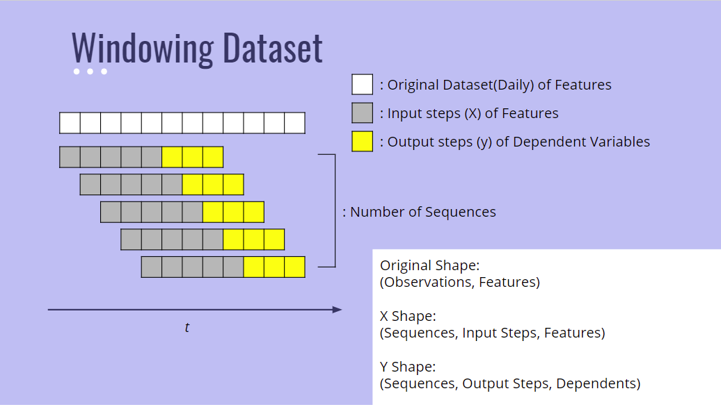
The training set needs to be windowed in order to be a valid input into the DCNN model. Essentially, the dataset will be separated into 2 matrices; X and y.
Initial dataframe shape: (Dates, Features)
X: (Number of Sequences, Input Steps, Input Features)
y: (Number of Sequences, Output Steps, Output Features)
I used 120 days of 77(7 regions x 11 features) features to output 41 days of 7 estimated fire area regions.
- 6 weather related means
- precipitation, humidity, soil water content, radiation, temperature, and wind speed
- 1 NDVI means
- 2 Surface Area Features
- 1 Estimated fire area
- 1 fire pixel counts
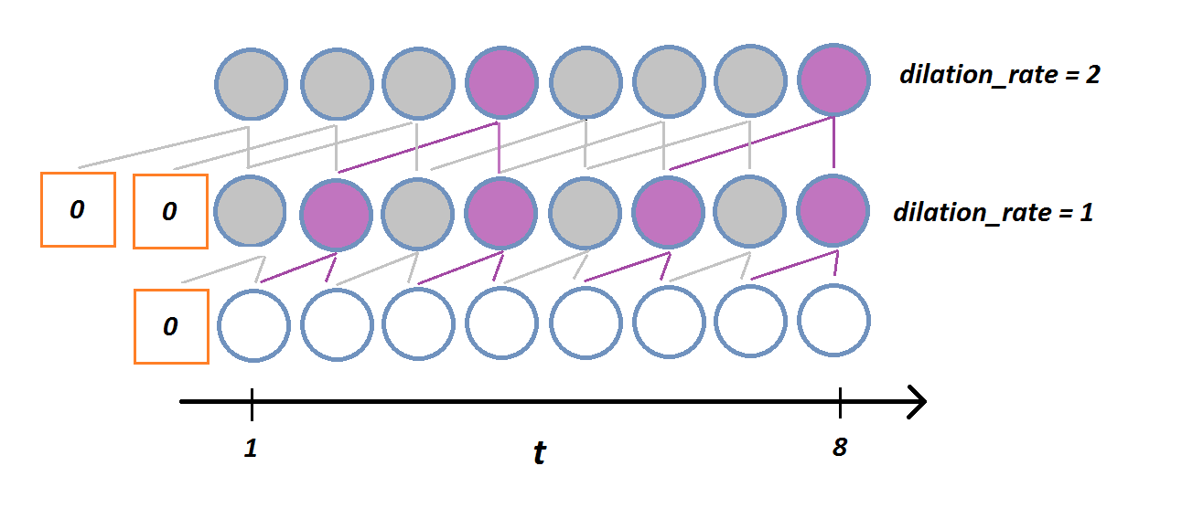
I utilized Conv1D layers with dilation to sling-shot 41 days of output. This would mean that the forecasted 41 days are independent of each other and this might not be necessarily what I want. However, the model may still give some promising results.
I utilized a WaveNet like architecture because of it's speed over traditional LSTM and GRU models. The convolution layers are created with sliding kernel inputs. Instead of taking all the inputs(120 days) to create the nodes of the first layer, Conv1D will take adjacent inputs to create each node of the layer.
In traditional Conv1D architecture, the number of hidden layers will increase one to one with the number of input steps. For example, if I have used 120 days of input with kernel size 2, the first layer will have 119 nodes the second layer 118 nodes and on.
To combat this problem, the creators of WaveNet utilized increasing dilations between each layer which essentially reduces the number of layers exponentially. Dilation skips nodes at an inputted rate and the unused nodes are not calculated.
The model had a mean absolute error of 21.07 and root mean squared error of 66.47 for the test set, December 01, 2020 - January 11, 2021. The final competition submission dates, February 01, 2021 - February 28, 2021, had a mean absolute error of 7.03 and rmse of 19.60. The stark contrast in evaluation scores may be explained due to the seasonal shift from December to February. The wildfires in December tend to be more robust due to warmer climate sthan February.
For further steps, I would like to first encorporate an autoregressive element to the model.
In addition, I would like to reaggregate the wildfires, weather, and vegetation statistics to county(administrative level 2) level or to custom hexagon shapes. This would make the dataset more coarse while still compressing enormous raster images.
