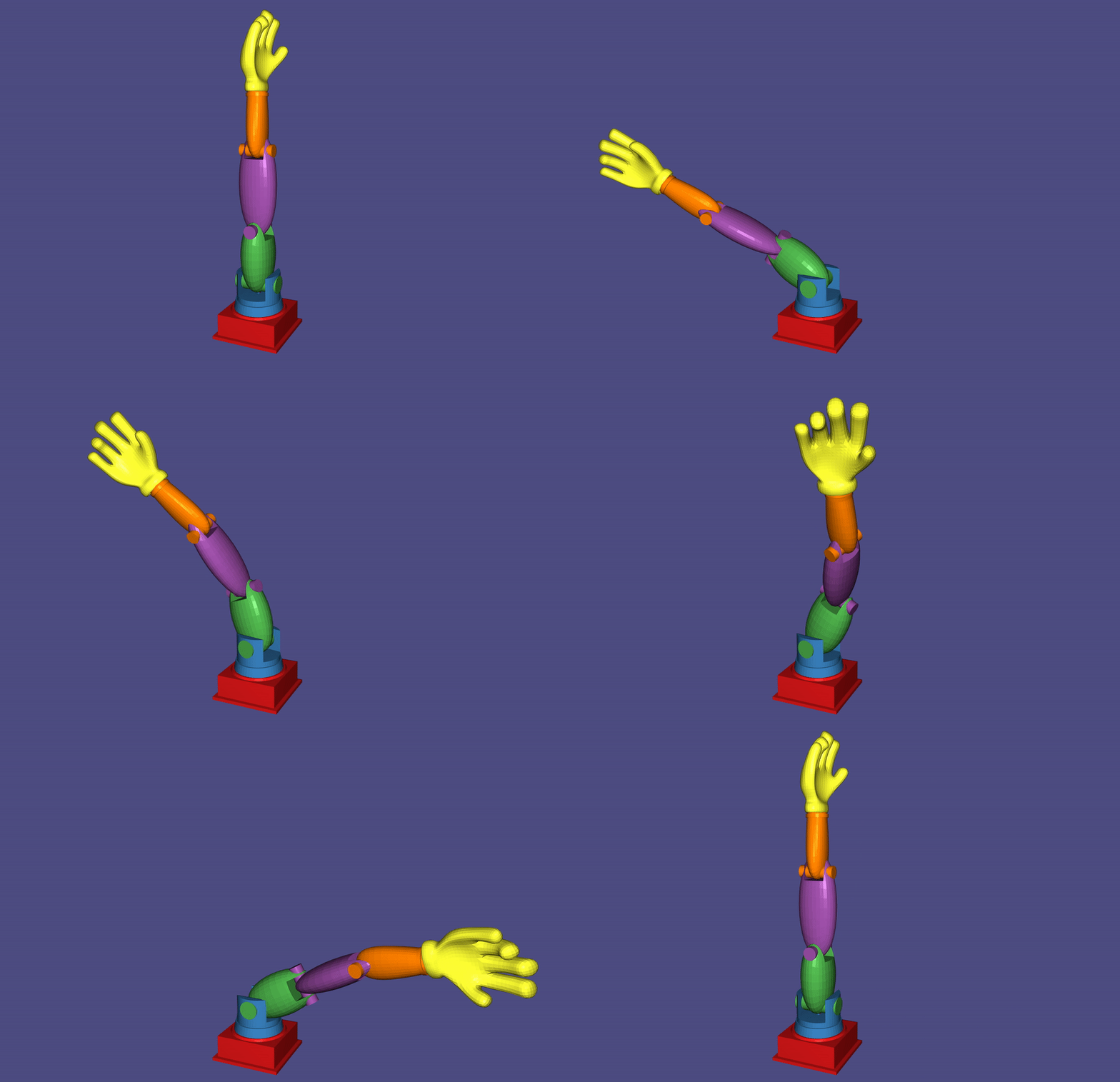
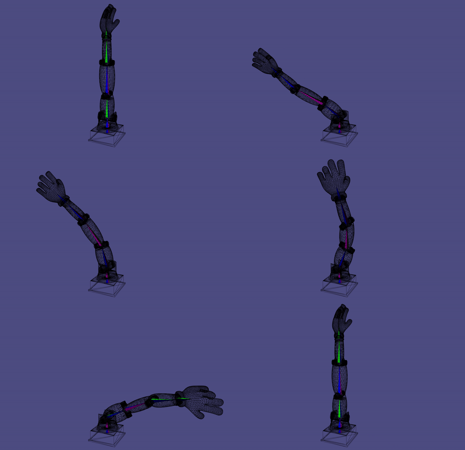
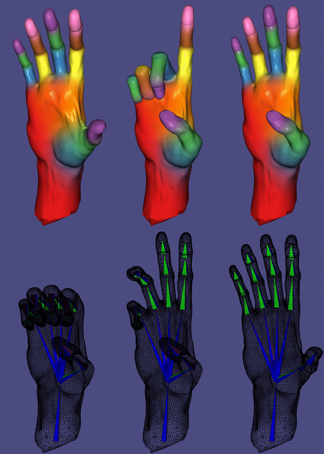
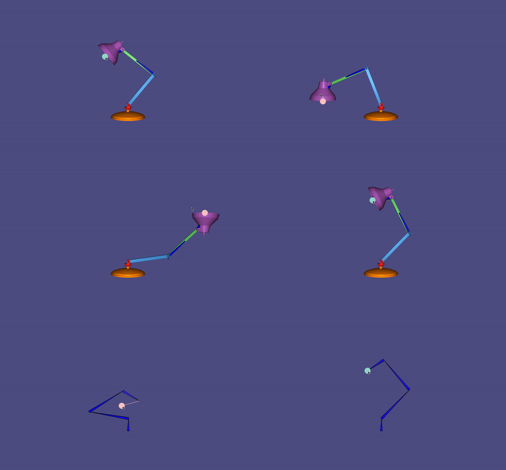
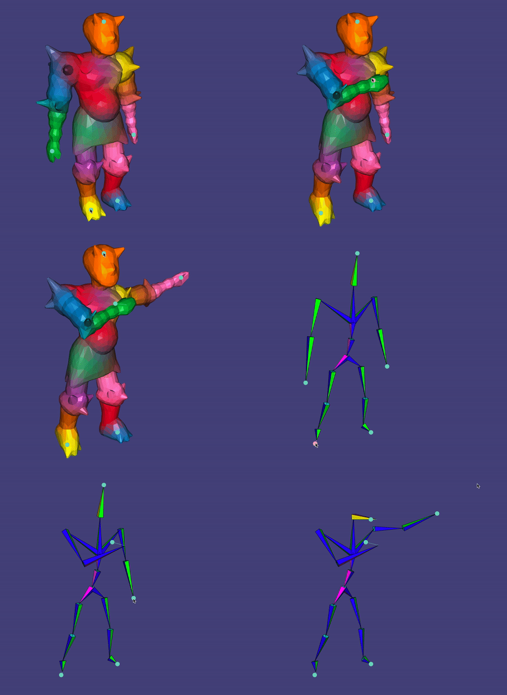
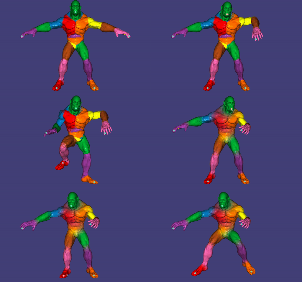
To get started: Clone this repository using
git clone --recursive http://github.com/alecjacobson/computer-graphics-kinematics.git
In this assignment we'll consider animating shapes rigged to an internal skeleton. The skeleton is a (graphical) user interface (UI) metaphor. A skeleton is a tree of rigid bones, not unlike the anatomical bones in a human or animal.
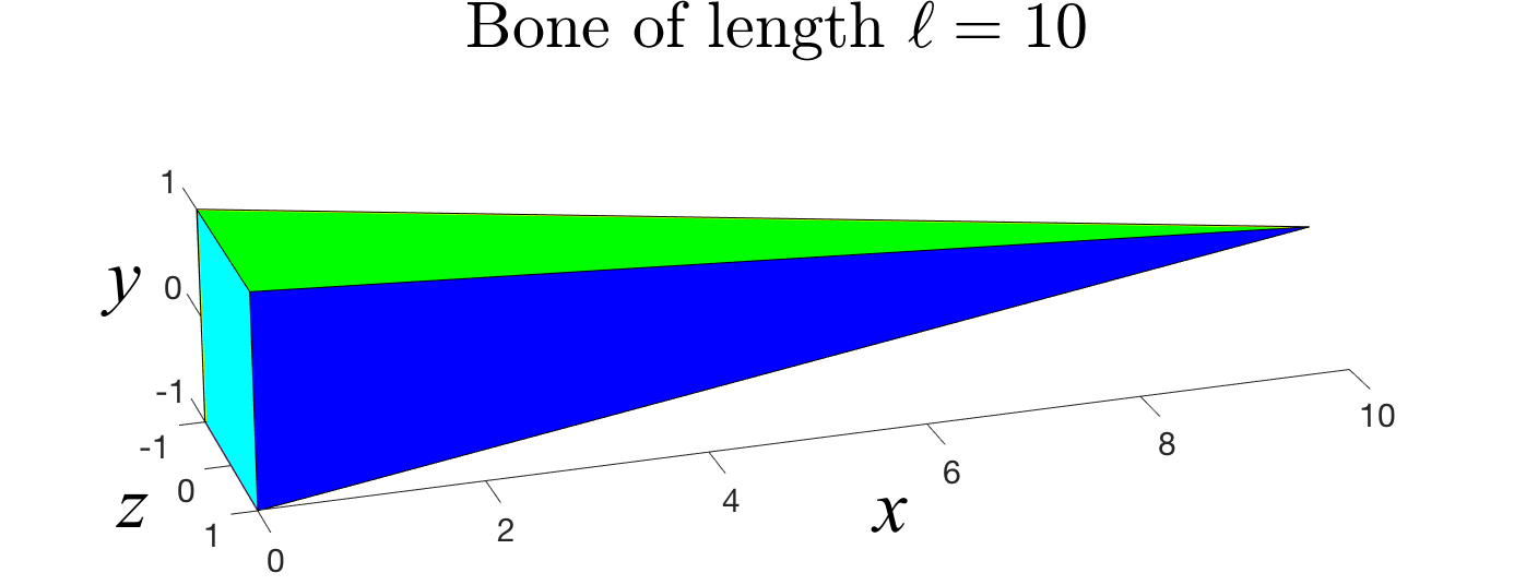
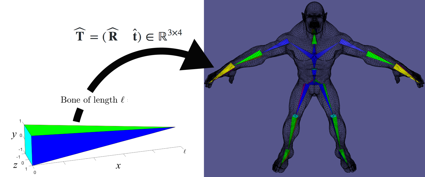
Each "bone" in the skeleton is really a UI widget for visualizing and controlling a 3D rigid transformation. A common visualization of 3D bone in computer graphics is a long, pointed pyramid shape. This reveals the twisting rotation as well as the tree hierarchy: the bone points toward its children.
Unlike anatomy where the brain triggers muscles to flex and pull the passive bones around, the bones of a skeleton rig will define the pose of a shape.
For each bone, we will consider three "states".
The "Canonical Bone" of length lies along the
-axis with its "tail" at
the origin
, its "tip" at
.
The bone is endowed with an
orientation or frame. This helps
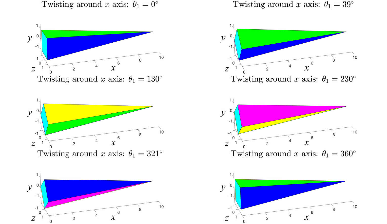
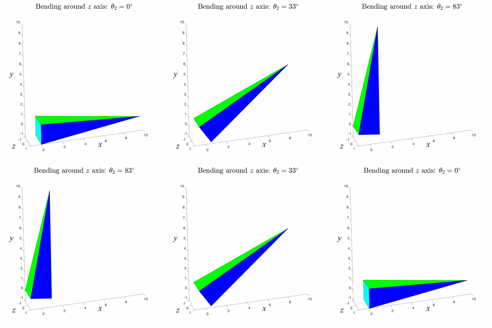
define a canonical twisting direction. We will define twisting as rotating about the -axis in the canonical frame.
For example, in this assignment, bending is accomplished by rotating about the
-axis in the canonical frame.
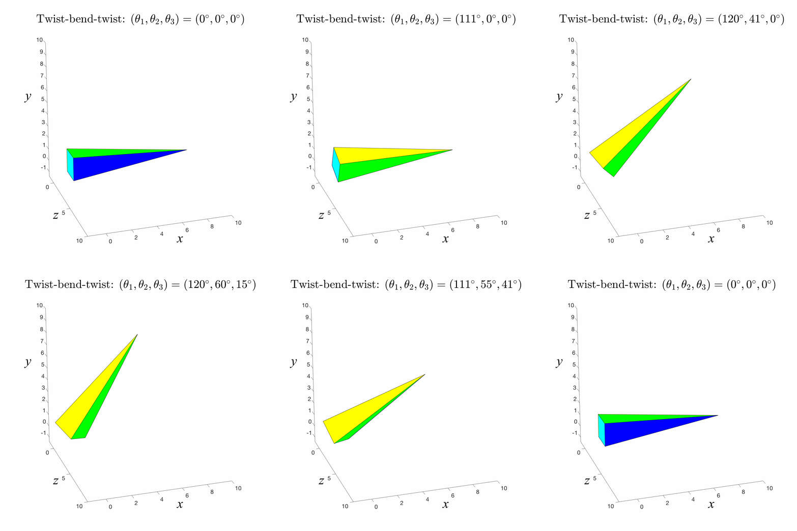
Composing a twist, bend and another twist spans all possible 3D rotations.
We call the three angles composed into a rotation this way, Euler angles (not to be confused with the homophonous Oiler angles).
To assemble a skeleton inside our shape will we map each bone from its
canonical bone to its position and orientation in the
undeformed model. Maintaining the rigidity of the bone, this means for each bone
there's a rigid transformation that places its tail and tip to the desired positions in the model.
We
use the convention that the "canonical tail" (the origin ) is mapped to
the "rest tail" inside the model. This means that the translation part of the
matrix
is simply the tail position,
:
The bone's
rotation is chosen so that the "canonical tip" maps to the "rest
tip"
:
Typically the "rest tail" of is coincident with the "rest tip" of its parent (if it exists):
This still leaves any amount of twisting of the bone. In the canonical frame,
we can think of this as pre-twisting the bone along the canonical -axis.
Clearly, twisting does not effect the ability to map the tail and tip to the
correct position. This twist is chosen so that canonical bending aligns with a
meaningful direction. For example, we may twist a tibia
(shinbone) bone so that canonical bending
around the
-axis means bending at the
knee.
Each rest transformation places its corresponding bone inside the
undeformed shape. The rest transformations do not measure any deformation of the
shape from its original position. Thus, the pose of each bone will be measured
relative to the "rest bone".
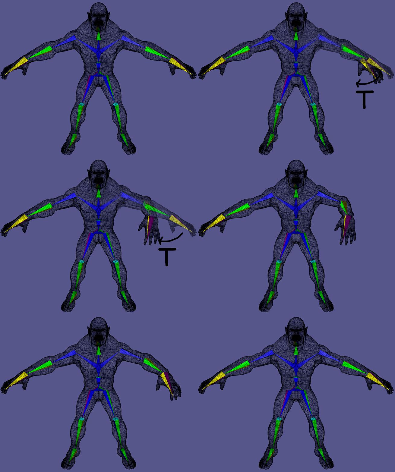
The final state to consider is when a bone is posed. That is, mapped to a new position and orientation from its rest state.
In general, each rest bone undergoes a rigid transformation ,
composed of a rotation
and a translation
, mapping each of its
rest points
to its corresponding posed postion
:
is expressed as a global mapping of any point in the rest reference frame
to its pose position. This makes it convenient for [blending transformations
(see below)][linearblendskinning], but it's not so obvious how to pick coherent
values for
. In particular, we would like each bone to rotate about its
parent's tip, but this position is determined by the parent's pose
transformation
, which in turn should rotate about the grandparent's tip
and so on.
One way to determine the rigid pose transformations for each
bone
in a skeleton is to aggregate relative rotations
between a bone
and its parent bone
in the skeletal tree.
The final transformation at some bone
deep in the skeletal tree is computed
via a recursive equation.
For each bone, (reading the effect of transformations right to left) we first
undo the map from canonical to rest (i.e., via inverting ), then
rotate by our relative rotation
, then map back to rest (via
). With our relative transformation accomplished, we continue up the
tree recursively
applying our parent's relative transformation, and our grandparent's and so on:
Question: Does using relative rotations ensure that bone tails stay coincident with parent tips?
As a base case, the root transformation can be defined to be the identity (no transformation) or the rigid transformation placing the object/character generally into a larger scene.
This has the great advantage that if the entire model is rotated or translated
at the root, the relative transformations still apply correctly. This property
holds locally, too. If bone controls the tibia
(shinbone) and
applies a bend at
the knee, then twisting and bending at the parent hip bone will naturally
compose with the knee bend.
It is convenient to express the relative rotations of each bone in the
canonical frame. We can utilize canonical twist-bend-twist
rotations (three Euler angles, ). Each bone's rotation
is conducted in its canonical frame and then brought through the rest frame
through a change of coordinates:
where the matrix is the rotation by
degrees around
the
-axis.
When implementing a skeleton, it is tempting to use a traditional tree data structure where each node (bone) contains a list of pointers to its children (other bones). However, by the right-to-left reading of the forward kinematics formulae above, it is more convenient to use a data structure where each node (bone) has a pointer to its (unique) parent (other bone). This is ridiculously named a Spaghetti Stack.
Question: What abstract data-structure is good for ensuring a parent's transformation
are computed before its child's
?
Hint: 🥞
To create a long animation, specifying three Euler angles for every bone for every frame manually would be too difficult. The standard way to determine the relative bone transformations for each frame is to interpolate values specified at a small number of "key" times during the animation. Linear interpolation will lead to a choppy, robotic animation (try this first!). Instead Catmull-Rom interpolation will produce a smooth animation. Fancier interpolation such as the Kochanek-Bartels method (called TCB in the book) allow better control of easing between key poses.
In this assignment, we will interpolate Euler angles directly. This works well
when only a single angle is changing at a time. However, Euler angles do not
provide easy movement in every rotational
direction. Euler angles model
rotations as twist-bend-twist. For our canonical bones, bending around the
-axis is easy, but bending around the
-axis requires first twisting by
and then "un"-twisting by
after bending.
So, for more complex interpolation of rotations, a different representation such as unit quaternions would be needed. This is outside the scope of this assignment.
In the [forward kinematics][forwardkinematics] model, the final position of the tip of a finger is determined by setting (manually or via interpolation) the relative transformations of each joint in the finger, the hand, the elbow, the shoulder, ... This indirect control makes it difficult to achieve basic poses. Instead, we can treat the problem of setting relative rotations of internal bones (shoulder, elbow, hand, ...) as an optimization problem where we try to minimize the distance between the tip of the finger and where we want it to be.
Stated mathematically, for a skeleton with bones, if we create a vector
stacking all the Euler angles of each bone vertically:
then we can ask for the best vector of angles . Best-ness must be quantified
by an cost/energy/obective-function
. This energy is typically first written
with respect to the (global, non-relative) pose positions of certains bones
(often the "tip" of a
leaf
bone of the skeletal tree, called an end
effector). For example, we
then we could design our energy to measure the squared distance between the pose
tip
of some bone
and a desired goal location
:
Using forward kinematics, we can express and in turn
with respect to
relative rotations:
where depends on
and
which depends on
. In this way our energy can be written as a
function of
:
We can design arbitrarily complex energies to satisfy our interaction needs. In
this assignment, we consider that there is a list of constrained end effectors
and our objective is that all selected end effectors
go to their prescribed locations (provided by the mouse-drag UI).
using the simple squared distance measure above.
So, over all choices of we'd like to optimize:
We will further constrain our problem by imposing
upper and lower bounds
on our angles . These correspond to joint limits. For example, the joint
limits of a hinge or elbow type joint may look like:
These would ensure that our joint cannot twist, and can only bend in one direction.
So our full optimization problem becomes
where stack lower/upper bounds correspondingly to
.
This type of minimization is non-trivial. Our energy is a quadratic sum of
squares in , but
is a non-linear function of
. In turn, this means to minimize
as
a function of
we must solve a non-linear least
squares problem.
We're faced with a bound constrained non-linear optimization problem. To solve
it, we will construct an initial guess and then iteratively improve the guess by
moving in a direction that decreases , after each step snap or project the
guess to stay within the bounds if necessary. This algorithm is called
projected gradient descent.
The idea behind gradient descent is intuitive: if you want to get to the bottom of a canyon, look at the ground and walk in the direction that goes downhill.
So, we iteratively take a step in the negative gradient direction of our
objective function :
Applying the chain rule, this iteration becomes
The change in tip positions with respect to joint angles
does not
depend on the choice of energy
. We call this matrix of changes the kinematic
Jacobian,
:
Written in terms of our step becomes,
Question: Can we take an arbitrarily large step
?
Hint: What if we just need to change
by a small, non-zero amount? What would chooing
do to
? What would that in turn do to
?
For sufficiently small , each step will decrease the objective energy
.
If the gradient of becomes zero, then we're at a stationary
point and likely at a minimum.
To ensure that our bounds are obeyed, after each step we need to project onto our constraints by snapping each value to its respective bound if necessary:
We'll refer to this as a projection filter acting on the entire vector :
The local gradient of a function can be very different from the "best" descent direction. The choice of
reflects how much we "trust" this direction. Unfortunately, if
is too large our iterations may diverge. If
is too small, we will have to do many iterations.
In order to find a better descent direction, let's assume we knew more about
. That is, suppose we also knew its second derivatives:
.
Given an initial guess
we're looking to find a change
so that
is a stationary point.
Starting with our equilibrium equation,
Plugging in a Taylor series expansion
and dropping higher order terms (
), we get:
where we call
the Hessian matrix.
Applying the differentiation by
we get a system of equations:
Solving for the change
we get:
So a raw Newton's method update would be:
If our Taylor series approximation was perfect (no high order terms in
; in otherwords
was quadratic), then Newton's method would be perfect: a single update immediately takes us to the minimum.
Newton's method is problematic for a number of reasons.
- We built our step purely based on the equations for a stationary point. Nothing says we won't get sent toward a maximum or saddle-point.
is often difficult or expensive to compute.
may be singular.
- Inverting
(even if possible) is often slow.
- Our system is built off a local approximation of
so the descent direction may still point in the wrong direction.
Since we're approximating
at every iteration anyway, we'll skirt many of these issues by considering various approximations of the Hessian matrix
. We'll never actually compute
.
The simplest approximation of
is the identity matrix
. Plugging this into our truncated Taylor series expansion above, our approximation would read:
and our step reduces to good ol' gradient descent:
Given that we have already computed first derivatives in the Jacobian
, an even better approximation for Hessian
than the identity
would be to use
. The resulting update becomes:
Unlike
,
is easy to compute if we're already computing
. It is guaranteed to be positive semi-definite and it is possible to invert or reliably pseudo-invert (
acting in place of
).
The descent directions are often significantly better than gradient descent. As a result this method, called Gauss-Newton, requires many fewer iterations to converge.
It still may try to descend in bad directions. In particular, for inverse kinematics, this Gauss-Newton method performs poorly if the desired positions are not reachable: over extending an arm. First the solution locks in place and then diverges. This happens when our Hessian approximation
starts misbehaving.
A good fix is to blend between the gradient descent and Gauss-Newton search directions. That is blend between
and
. This is called the Levenberg-Marquadt algorithm.
But how do we compute the kinematic Jacobian ? Since each entry in
is
the result of forward kinematics and not just a math expression, it's not
immediately obvious how to determine its derivatives. However, a derivative is
nothing more than the limit of a small change output divided by a small change
in the input:
where is a vector of zeros except a 1 at location
.
We can numerically approximate this limit by fixing to a small value (e.g.,
). This is called the finite
difference approximation:
For inverse kinematics, we will need to compute once for each
Euler angle of each bone
. This requires
calls to our forward kinematics
function (each with a slightly different input), which is in turn
. This
makes the total cost
to fill in our
matrix.
Forward differencing requires
evaluations but doesn't require us to change our code for function evaluation at all: we just evaluate it. If we're willing to sprinkle some special types on top of our code (but otherwise leave in all the sub-routine calls, if statements, for loops, etc.), we could use automatic differentiation to compute
.
The are two extremes when it comes to autodiff: forward mode and backward mode.
Forward mode works like finite differencing, except the perturbation to the differentiation variable is symbolic and derivatives are tracked through each basic operation (
+,-,sin,etc.): the total computational cost to constructis again
.
Backward mode works by pushing each function call and basic operation onto a list. Derivatives for all variables are then computed as we pop backward through the evaluation: identical to how we read right-to-left on our recursive kinematics formula. This means we compute derivatives with respect to all variables
in a single backwards evaluation. The total cost is only
to fill
.
Whether we're using gradient descent, Newton's method or Gauss-Newton, we a
generally attempting improving our guess by iteratively moving in a descent
direction , followed by projecting onto constraints:
Despite our best efforts, this step is not guaranteed to actually decrease
our energy . We can think of the descent direction
as defining a line (or really
a ray) and we'd like to find a positive amount
to move along this line that actually
does decrease the energy:
While there exists an optimal step , we don't want to spend too long finding
it as we would be better off spending our computational efforts improving the
descent direction for the next step. So, starting with a large value
(e.g., 10,000), we decrease
by a constant factor (e.g.,
) until our
inequality passes.
Depending on the configuration, it may or may not be possible to exactly satisfy
the constraints (i.e., ). But after many iterations, the solution should
converge to a local minimum
(i.e.,
, but
). In our assignment, a thin line will appear if
the user-given constraint is not coincident with the end-effector tip position.
So far we have only discussed bones floating and moving around in space. Ultimately, we would like to deform interesting models: for example, animals and characters. Unlike robots or mechanical objects, the animals tend to deform smoothly, even near joints: an elbow does not tear into two rigid parts when bent. Instead, the skin around the elbow stretches and smoothly warps. Skin closer to the forearm deforms more like the rigid rotation and translation of the forearm, and likewise the skin near the upper arm deforms like the rigid upper arm bone. In between, we see a smooth transition or blend.
To approximate this smooth blending quickly on the computer, we begin with a 3D
triangle mesh in its "rest" position. The "rest bones" are embedded inside of
this model. Each vertex of the mesh is assigned a weight
for each
bone
corresonding to how much it is "attached" to that bone on a scale of 0%
to 100%. Generally, if the rest position of the vertex
is nearer to
a bone
then its weight
will be larger. A vertex in the middle of
the elbow may have a weight of 50% for the upper arm and 50% the forearm and
0% for all other bones (toes, fingers, legs, spine, etc.).
Smoothly varying weights produce a smooth deformation. In constrast, piecewise-constant weights lead to a piece-wise rigid deformation.
The "pose" position of this vertex
will be computed as a weighted
average or linear combination of each bone's pose transformation
applied
to the vertex's rest position
:
Question: What happens to per-vertex normals after applying a skinning deformation?
Hint: 🤯
Linear blend skinning has many defects. Good "rigging artists" can mitigate these by carefully painting (yes, painting) weight functions and position the rest bones. However, some of the linear blend skinning defects are theoretical: most notably problems that occur by averaging rotations as matrices.
Question: What transformation matrix do you get if you compute:
?
Eigen::Affine3dEigen::AngleAxis#include <Eigen/Geometry>- c++ lambda functions and capturing
#include <functional>
igl::lbsigl::forward_kinematics
This README file is too complex for texify to render. Use readme2tex locally to render the TeX to SVGs.
python -m readme2tex --output README.md README.tex.md --nocdn
sed -i 's/invert_in_darkmode\"/invert_in_darkmode\&sanitize=true\"/g' README.md
