/geometry-processing-parameterization

Parameterization assignment for Geometry Processing course

Primary LanguageC++Mozilla Public License 2.0MPL-2.0

Geometry Processing – Parameterization

To get started: Clone this repository with

git clone --recursive http://github.com/alecjacobson/geometry-processing-parameterization.git

Installation, Layout, and Compilation

See introduction.

Execution

Once built, you can execute the assignment from inside the build/ by running on a given mesh:

./parameterization [path to mesh with boundary.obj]

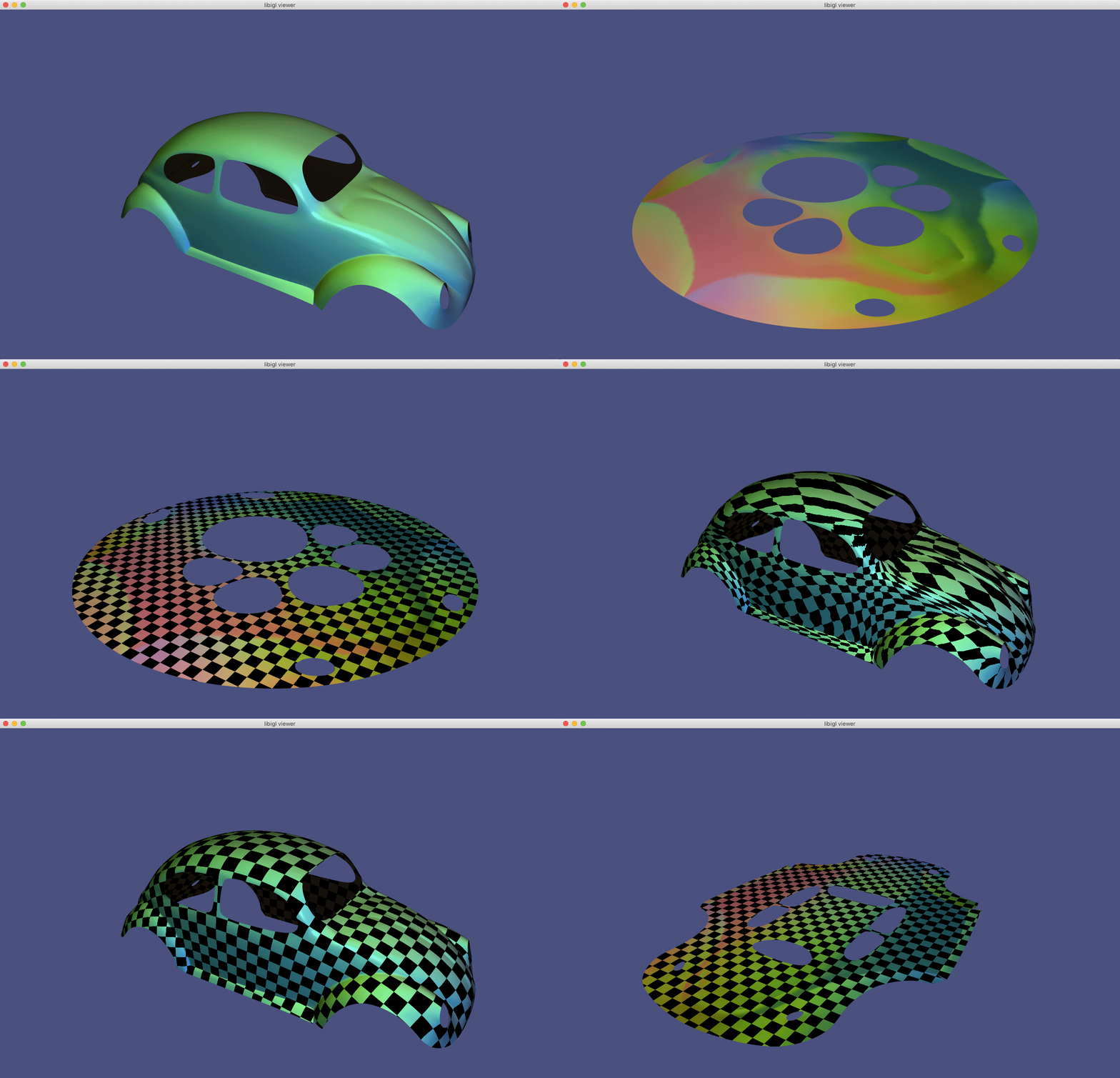
When your app is implemented correctly you'll be able to cycle through viewing the mesh, viewing the parameterization, toggling the checkerboard pattern and switching between parameterization methods.

Background

In this assignment we will explore how to flatten a surface embedded (or even just immersed) in $\mathbb{R}^3$ to the flat plane (i.e. $\mathbb{R}^2$).

This process is often referred to as parameterization because the two-dimensional coordinate system of the flattened mesh can now be interpreted as a parameterization of the 3D surface.

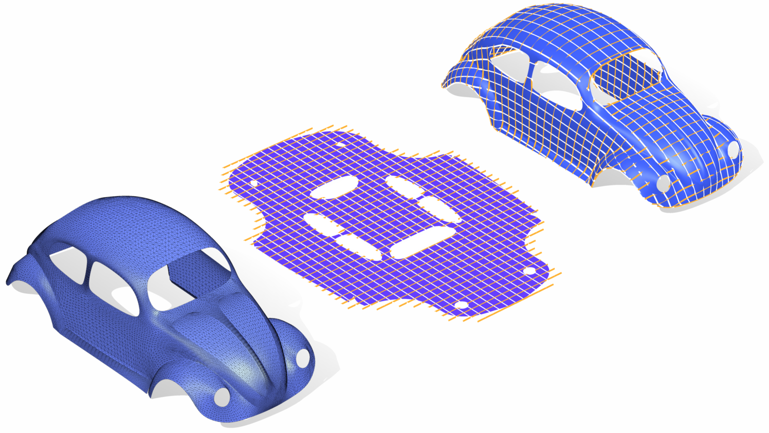
A triangle mesh of a VW Beetle is parameterized by flattening the mesh to the $uv$ -plane. There the $u$- and $v$- coordinates (orange and white lines) can be directly interpreted as a parameterization of the surface.

In this assignment, we are given a representation of the surface in 3D as a triangle mesh with a list of $n$ vertex positions $\mathbf{V} \in \mathbb{R}^{n \times 3}$, so then the goal is to assign $uv$ coordinates to each vertex $\mathbf{U} \in \mathbb{R}^{n \times 2}$.

In general, a 3D surface cannot be flattened onto the plane without distortion. Some parts of the surface will have to be stretched and other squished. Surfaces with topological handles or without a boundary must be cut.

Mass-spring methods

If we view our triangle mesh surface as a simple graph then the surface flattening problem reduces to graph drawing. Distortion can be measured in terms of the relative change in lengths between neighboring vertices.

We can pose the graph drawing problem as an optimization over node locations so that the lengths between neighboring vertices are minimized:

$$ \mathop{\text{min}}_\mathbf{U} \sum\limits_{\{i,j\} \in \mathbf{E}} || \mathbf{u}_i - \mathbf{u}_j||^{2}, $$

where $\mathbf{E}\in \{1,\ldots ,n\}^{k \times 2}$ holds a list of edge indices into $\mathbf{V}$. This energy has a physical interpretation as the potential energy of mass-spring system. Each edge represents a spring with zero rest length, all springs have uniform stiffness, and all vertices have equivalent (unit) mass.

Without additional constraints, this minimization has a trivial solution: map all vertices to the same point, e.g., $\mathbf{u}_i = (0\ 0),\ \forall i$.

We can avoid this by fixing the mapping of certain vertices. If we choose these fixed vertices arbitrarily we will in general get overlaps in the flattening. For graph drawing this means that edges cross each other; for surface parameterization this means that multiple triangles cover the same patch of the $uv$-plane and some of those triangles are upside down. This problem is often referred to as fold overs or lack of injectivity.

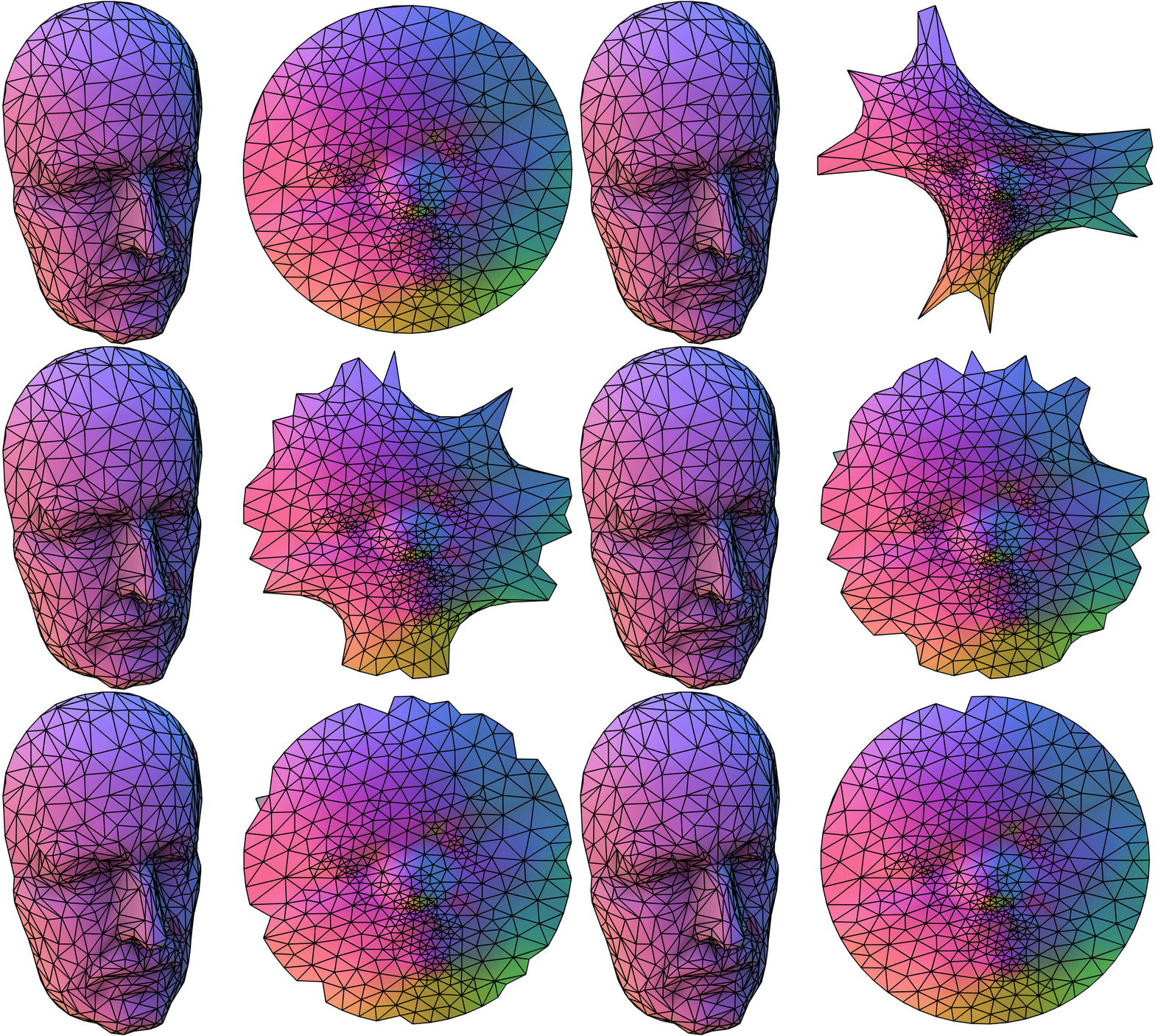
The face of Max Planck is parameterized using a mass-spring system. More and more vertices are fixed explicitly along the boundary. With only a few fixed vertices there are severe overlaps and degeneracies in the interior. When the entire boundary is fixed to the circle, there are no overlaps.

In 1963, Tutte showed that if the boundary of a disk-topology mesh is fixed to a convex polygon (and all spring stiffness are positive) then minimizing the energy above will result in an injective (i.e., fold-over-free) flattening.

While avoiding fold-overs is important, Tutte-style mappings suffer from a couple problems.

If uniform spring stiffness are used, then the mapping in the $uv$ domain will try to make all edges the same length. Combined with the boundary constraints, the flattened mesh will have smoothly varying edge-lengths and near-equilateral triangles regardless of the triangles shapes and sizes on the surface mesh.

The Tutte embedding of the 3D Ogre mesh leads to severe distortion. Overlaying a checkerboard pattern on the 2D domain and visualizing it on the 3D surface shows the wobbliness of the non-smooth mapping and stretching.

We can try to remedy this by introducing a non-uniform weight or spring stiffness $w_{ij}$ for each edge $\{i,j\}$:

$$ \mathop{\text{min}}_\mathbf{U} \sum\limits_{\{i,j\} \in \mathbf{E}} w_{ij} || \mathbf{u}_i - \mathbf{u}_j||^{2}. $$

For example, we could weigh the distortion of shorter edges (on the 3D mesh) more than longer ones: $w_{ij} = 1/|| \mathbf{v}_i - \mathbf{v}_j|| $. See "Parametrization and smooth approximation of surface triangulations" [Floater 1996]. This will at best help tame length distortion. The "shapes" (i.e., aspect ratios) of triangles will only be indirectly preserved. We need a way to discourage area distortion and angle distortion.

To do this, let's write the energy minimization problem above in matrix form:

$$ \mathop{\text{min}}_\mathbf{U} \frac12 \mathop{\text{tr}}{\left(\mathbf{U}^{\mathsf T} \mathbf{L} \mathbf{U}\right)}, $$

where $\mathbf{L} \in \mathbb{R}^{n \times n}$ is a sparse matrix with:

$$ L_{ij} = \begin{cases} w_{ij} & \text{ if $i\ne j$ and $\exists \{ij\} \in \mathbf{E}$, }\\ -\sum\limits_{\ell\ne i} L_{i\ell} & \text{ if $i = j$, or } \\ 0 & \text{ otherwise} \end{cases}. $$

What's up with the $\mathop{\text{tr}}{\left(\right)}$ in the energy?

The degrees of freedom in our optimization are a collected in the matrix $\mathbf{U} \in \mathbb{R}^{n\times 2}$ with two columns. The energy is written as the trace of the quadratic form (a.k.a. matrix) $\mathbf{Q} \in \mathbb{R}^{n\times n}$ applied to $\mathbf{U}$. In effect, this is really applying $\mathbf{Q}$ to each column of $\mathbf{U}$ independently and summing the result:

$$ \begin{align*} \mathop{\text{tr}}{\left(\mathbf{U}^{\mathsf T} \mathbf{Q} \mathbf{U}\right)} &= \\ &= \mathop{\text{tr}}{\left(\mathbf{U}^{\mathsf T} \mathbf{Q} \mathbf{U}\right)} \\ &= {\mathop{\text{tr}}\left( { \left[\begin{array}{c} \mathbf{U}_1^{\mathsf T}\\ \mathbf{U}_2^{\mathsf T} \end{array}\right] \mathbf{Q} [\mathbf{U}_1 \mathbf{U}_2] } \right)} \\ &= {\mathop{\text{tr}}\left( \begin{bmatrix} \mathbf{U}_1^{\mathsf T} \mathbf{Q} \mathbf{U}_1 & \mathbf{U}_1^{\mathsf T} \mathbf{Q} \mathbf{U}_2 \\ \mathbf{U}_2^{\mathsf T} \mathbf{Q} \mathbf{U}_1 & \mathbf{U}_2^{\mathsf T} \mathbf{Q} \mathbf{U}_2 \end{bmatrix} \right)} \\ &= \mathbf{U}_1^{\mathsf T} \mathbf{Q} \mathbf{U}_1 + \mathbf{U}_2^{\mathsf T} \mathbf{Q} \mathbf{U}_2. \end{align*} $$

The benefits of energies written as the trace of a quadratic form applied to a matrix include: 1) each column can be optimized independently (assuming constraints are also separable by column), and this is often the case when columns correspond to coordinates (u, v, etc.); and 2) the quadratic form for each columns is the same (the same $\mathbf{Q}$). For quadratic energy minimization, this means that we can precompute work (e.g., Cholesky facotorization) on $\mathbf{Q}$ and take advantage of it for solving with $\mathbf{U}_1$ and $\mathbf{U}_2$ and we might even solve in parallel.

Dirichlet energy

We should immediately recognize this sparsity structure from the discrete Laplacians considered in the previous assignments. If $w_{ij} = 1$, then $\mathbf{L}$ is the uniform Laplacian (a.k.a., graph Laplacian). If $w_{ij}$ is based on edge-lengths, then $\mathbf{L}$ corresponds to a physical static equilibrium problem for a linear spring system.

But we have more information than edges: we know that our graph is really a discrete representation of a two-dimensional surface. Wobbliness distortions in the parameterization correspond to high variation in the $u$ and $v$ functions over the surface.

We can model the problem of parametrization as an energy minimization of the variation in the $u$- and $v$-coordinate functions over the surface $\mathbf{S}$:

$$ \mathop{\text{min}}_{u,v} \int_\mathbf{S} || {\nabla}u||^{2} + || {\nabla}v||^{2} \ dA. $$

This familiar energy is called the Dirichlet energy.

We may discretize this problem immediately using piecewise linear functions spanned by $u$ and $v$ values at vertices. This corresponds to using the cotangent Laplacian as $\mathbf{L}$ in the discrete minimization problem above.

In the smooth setting, minimizing the variation of $u$ and $v$ will lead to an injective mapping if the boundary is constrained to a closed convex curve. In the discrete setting, poor triangle shapes in the original 3D mesh could lead to negative cotangent weights $w_{ij}$ so the positive stiffness weight assumption of Tutte's theorem is broken and fold-overs might occur. Keep in mind that positive weights are a sufficient condition for injectivity, but this does not imply that having a few negative weights will necessarily cause a fold-over. Even so, Floater proposes an alternative discrete Laplacian in "Mean value coordinates" in 2003 that retains some nice shape-preserving properties without negative weights.

Modeling distortion as an integral of variation over the given 3D surface is going in the right direction, but so far we are treating $u$ and $v$ separately. Intuitively $u$ and $v$ cannot "talk" to one-another during optimization. There's no reason to expect that they will be able to minimize area distortation and angle distortion directly. For that we will need to consider $u$ and $v$ simultaneously.

Least Squares Conformal Mappings

We can reason about distortion in terms of differential quantities of the mapping from $\mathbf{S}$ to $\mathbb{R}^{2}$. Now, ultimately we are trying to parametrize $\mathbf{S}$ using the $u$ and $v$ coordinate functions spanning $\mathbb{R}^2$, but in order to describe energies over these unknown functions we will assume (without explicitly using) that we have a parameterization of $\mathbf{S}$ (e.g., with coordinates $x$ and $y$). This way we can write about small changes in the mapping function $u$ with respect to moving a small amount on the surface of $\mathbf{S}$ (small changes in $x$ and $y$).

Area distortion

We would like that regions on $\mathbf{S}$ have a proportionally similarly sized region under the $u$, $v$ mapping to $\mathbb{R}^{2}$. On an infinitesimal scale, a small change in $x$ and $y$ on $\mathbf{S}$ should incur an equally small change in $u$ and $v$. In other words, the determinant of the Jacobian of the mapping should be one:

$$ \left| \begin{array}{cc} \frac{\partial u}{\partial x} & \frac{\partial u}{\partial y} \\ \frac{\partial v}{\partial x} & \frac{\partial v}{\partial y} \end{array} \right| = 1, $$

where $| \mathbf{X} | = \det{\mathbf{X}}$ for a square matrix $\mathbf{X}$.

The determinant of the Jacobian of a mapping corresponds to the scale factor by which local area expands or shrinks. This quantity also appears during integration by substitution when multivariate functions are involved.

It is tempting to try to throw this equality into a least squares energy an minimize it. Unfortunately the determinant is already a quadratic function of $u$ and $v$ so a least-squares energy would be quartic and minimizing it would be non-trivial. In the deformation assignment, we consider area-distortion directly when looking for "as-rigid-as-possible" mappings. This idea can also be applied to parameterization (also leading to a non-linear optimization). But for this assignment, let us put aside area distortion and focus instead on angle or aspect-ratio distortion.

Angle distortion

We would also like that local regions on $\mathbf{S}$ are parameterized without shearing. This ensures that two orthogonal directions on the surface $\mathbf{S}$ correspond to two orthogonal directions on the parameteric plane $\mathbb{R}^{2}$. We can capture this by requiring that a small change in the $x$ and $y$ directions on $\mathbf{S}$ corresponds to equal magnitude, small changes in $u$ and $v$ in perpendicular directions:

$$ \begin{align*} {\nabla}u &= {\nabla}v^\perp \\ &\downarrow \\ \begin{bmatrix} \frac{\partial u}{\partial x} \\ \frac{\partial u}{\partial y} \\ \end{bmatrix} &= \begin{bmatrix} \frac{\partial v}{\partial y} \\ -\frac{\partial v}{\partial x} \\ \end{bmatrix} \end{align*} $$

where $\mathbf{x}^\perp$ indicates the vector $\mathbf{x}$ rotated by $90^\circ$.

By enlisting complex analysis, we can reinterpret the mapping to the real plane $\mathbb{R}^{2}$ as a mapping to the complex plane $\mathbb{C}$. The angle preservation equality above corresponds to the Cauchy-Riemann equations. Complex functions that satisfy these equations are called conformal maps.

This equality is linear in $u$ and $v$. We can immediately build a quadratic energy that minimizes deviation from satisfying this equation over the surface $\mathbf{S}$ in a least squares sense:

$$ \mathop{\text{min}}_{u,v} \frac12 \int_\mathbf{S} || {\nabla}u - {\nabla}v^\perp||^{2} \ dA. $$

This energy was employed for surface parameterization of triangle meshes as early as "Intrinsic parameterizations of surface meshes" [Desbrun et al. 2002] and "Least squares conformal maps for automatic texture atlas generation" [Lévy et al. 2002]. Written in this form, it's perhaps not obvious how we can discretize this over a triangle mesh. Let us massage the equations a bit, starting by expanding the squared term:

$$ \int_\mathbf{S} \left(\frac12 || {\nabla}u||^{2} + \frac12 || {\nabla}v||^{2} - {\nabla}u \cdot {\nabla}v^\perp \right)\ dA. $$

We should recognize the first two terms as the Dirichlet energies of $u$ and $v$. The third term is at first glance not familiar. Let's massage it a bit by expanding the gradient and dot product:

$$ \begin{align*} \int_\mathbf{S} {\nabla}u \cdot {\nabla}v^\perp \ dA &= \\ \int_\mathbf{S} \left( \begin{array}{r} \frac{\partial u}{\partial x} \\ \frac{\partial u}{\partial y} \\ \end{array}\right)\cdot \left( \begin{array}{r} \frac{\partial v}{\partial y} \\ -\frac{\partial v}{\partial x} \\ \end{array} \right) \ dA &= \\ \int_\mathbf{S} \left| \begin{array}{cc} \frac{\partial u}{\partial x} & \frac{\partial u}{\partial y} \\ \frac{\partial v}{\partial x} & \frac{\partial v}{\partial y} \end{array} \right| \ dA &= \int_{\left(\begin{array}{c}u(\mathbf{S}) \\ v(\mathbf{S}) \end{array}\right)} 1 \ dA, \end{align*} $$

where we end up with the integrated determinant of the Jacobian of the $u$ and $v$ mapping over $\mathbf{S}$. By the rules of integration by substitution, this is equivalent to integrating the unit density function over the image of the mapping, i.e., the signed area of the flattened surface. If we apply divergence theorem we can convert this area integral into a boundary integral:

$$ \int_{\left(\begin{array}{c}u(\mathbf{S}) \\ v(\mathbf{S}) \end{array}\right)} 1 \ dA = \frac12 \oint_{\partial \left(\begin{array}{c}u(\mathbf{S}) \\ v(\mathbf{S}) \end{array}\right)} \mathbf{u}(s)\cdot \mathbf{n}(s) \ ds, $$

where $\mathbf{n}$ is the unit vector pointing in the outward direction along the boundary of the image of the mapping.

If we discretize $u$ and $v$ using piecewise-linear functions then the boundary of the mapping will also be piecewise linear and the boundary integral for the vector area is given by the sum over all boundary edges of the integral of the position vector $\mathbf{u}$ dotted with that edge's unit normal vector:

$$ \begin{align*} \frac12 \oint_{\partial (\mathbf{u}(\mathbf{S}))} \mathbf{u}(s)\cdot \mathbf{n}(s) \ ds &= \frac12 \sum\limits_{{i,j} \in \partial \mathbf{S}} \int_0^1 (\mathbf{u}_i + t(\mathbf{u}_j - \mathbf{u}_i))\cdot \frac{(\mathbf{u}_j-\mathbf{u}_i)^\perp}{|| \mathbf{u}_j - \mathbf{u}_i|| } \frac{ds}{dt}\ dt \\ &= \frac12 \sum\limits_{{i,j} \in \partial \mathbf{S}} \int_0^1 (\mathbf{u}_i + t(\mathbf{u}_j - \mathbf{u}_i))\cdot \frac{(\mathbf{u}_j-\mathbf{u}_i)^\perp}{|| \mathbf{u}_j - \mathbf{u}_i|| } || \mathbf{u}_j - \mathbf{u}_i|| \ dt \\ &= \frac12 \sum\limits_{{i,j} \in \partial \mathbf{S}} \int_0^1 \mathbf{u}_i\cdot (\mathbf{u}_j-\mathbf{u}_i)^\perp dt \\ &= \frac12 \sum\limits_{{i,j} \in \partial \mathbf{S}} | \mathbf{u}_i\ \mathbf{u}_j |, \end{align*} $$

where finally we have a simply quadratic expression: sum over all boundary edges the determinant of the matrix with vertex positions as columns. This quadratic form can be written as $\mathbf{U}^{\mathsf T} \mathbf{A} \mathbf{U}$ with the vectorized $u$- and $v$-coordinates of the mapping in $\mathbf{U} \in \mathbb{R}^{2n}$ and $\mathbf{A} \in \mathbb{R}^{2n \times 2n}$ a sparse matrix involving only values for vertices on the boundary of $\mathbf{S}$.

Achtung! A naive implementation of $\frac12 \sum \limits_{{i,j} \in \partial \mathbf{S}} | \mathbf{u}_i \mathbf{u}_j |$ into matrix form $\mathbf{U}^{\mathsf T} \mathbf{A} \mathbf{U}$ will likely produce an asymmetric matrix $\mathbf{A}$. From a theoretical point of view, this is fine. $\mathbf{A}$ just needs to compute the signed area of the flattened mesh. However, from a numerical methods point of view we will almost always need our quadratic coefficients matrix to be symmetric. Fortunately, when a matrix is acting as a quadratic form it is trivial to symmetrize. Consider we have some asymmetric matrix $\tilde{\mathbf{A}}$ defining a quadratic form: $\mathbf{x}^{\mathsf T} \tilde{\mathbf{A}} \mathbf{x}$. The output of a quadratic form is just a scalar, so it's equal to its transpose:

$$ \mathbf{x}^{\mathsf T} \tilde{\mathbf{A}} \mathbf{x} = \mathbf{x}^{\mathsf T} \tilde{\mathbf{A}}^{\mathsf T} \mathbf{x}. $$

These are also equal to their average:

$$ \mathbf{x}^{\mathsf T} \tilde{\mathbf{A}} \mathbf{x} = \mathbf{x}^{\mathsf T} \underbrace{\frac12 (\tilde{\mathbf{A}} + \tilde{\mathbf{A}}^{\mathsf T})}_{\mathbf{A}} \mathbf{x} = \mathbf{x}^{\mathsf T} \mathbf{A} \mathbf{x} $$

Putting this together with the Dirichlet energy terms, we can write the discrete least squares conformal mappings minimization problem as:

$$ \mathop{\text{min}}_{\mathbf{U} \in \mathbb{R}^{2n}} \mathbf{U}^{\mathsf T} \underbrace{ \left( \left( \begin{array}{rr} \mathbf{L} & 0 \\ 0 & \mathbf{L} \end{array} \right) - \mathbf{A} \right) }_{\mathbf{Q}} \mathbf{U}, $$

where $\mathbf{L} \in \mathbb{R}^{n \times n}$ is the Dirichlet energy quadratic form (a.k.a. cotangent Laplacian) and $\mathbf{Q} \in \mathbb{R}^{2n \times 2n}$ is the resulting (sparse) quadratic form.

Free boundary

Similar to the mass-spring methods above, without constraints the least squares conformal mapping energy will also have a trivial solution: set $\mathbf{U}$ to a single point.

To avoid this solution, we could "fix two vertices" (as originally suggested by both [Desbrun et al. 2002] and [Lévy et al. 2002]). However, this will introduce bias. Depending on the two vertices we choose we will get a different solution. If we're really unlucky, then we might choose two vertices that the energy would rather like to place near each other and so placing them at arbitrary positions will introduce unnecessary distortion (i.e., high energy).

Instead we would like natural boundary conditions (not to be confused with Neumann boundary conditions). Natural boundary conditions minimize the given energy in the absence of explicit (or essential) boundary conditions. Natural boundary conditions are convenient if we discretize the energy before differentiating to find the minimum. If our discretization is "good", then natural boundary conditions will fall out for free (natural indeed!).

To obtain natural boundary conditions without bias and avoid the trivial solution, we can require that the solution:

  1. minimizes the given energy,
  2. has non-zero norm, and
  3. is orthogonal to trivial solutions.

Let's break these down. The first requirement simply ensures that we're still minimizing the given energy without monkeying around with it in any way.

The second requirement adds the constraint that the solution $\mathbf{U}$ has unit norm:

$$ \int_\mathbf{S} || \mathbf{u}||^{2} \ dA = 1. $$

In our discrete case this corresponds to:

$$ \mathbf{U}^{\mathsf T} \underbrace{\left(\begin{array}{cc}\mathbf{M} & 0 \\ 0 & \mathbf{M} \end{array}\right)}_{\mathbf{B}} \mathbf{U} = 1, $$

where $\mathbf{M} \in \mathbb{R}^{n \times n}$ is the mass matrix for a piecewise-linear triangle mesh and $\mathbf{B} \in \mathbb{R}^{2n \times 2n}$ is the sparse, square constraint matrix

This is a quadratic constraint. Normally that would be bad news, but this type of constraint results in a well-studied generalized Eigen value problem.

Generalized Eigenvalue problem

Consider a discrete quadratic minimization problem in $\mathbf{v} \in \mathbb{R}^n$:

$$ \mathop{\text{min}}_{\mathbf{v}} \frac12 \mathbf{v}^{\mathsf T} \mathbf{A} \mathbf{v} \text{ subject to } \mathbf{v}^{\mathsf T} \mathbf{B} \mathbf{v} = 1, $$

where $\mathbf{A},\mathbf{B} \in \mathbb{R}^{n \times n}$ are positive semi-definite matrices.

We can enforce this constraint via the Lagrange multiplier method by introducing the scalar Lagrange multiplier ${\lambda}$ and looking for the saddle-point of the Lagrangian:

$$ \mathcal{L}(\mathbf{v},{\lambda}) = \frac12 \mathbf{v}^{\mathsf T} \mathbf{A} \mathbf{v} + {\lambda} (1 - \mathbf{v}^{\mathsf T} \mathbf{B} \mathbf{v} ). $$

This occurs when $\partial \mathcal{L}/\partial \mathbf{v} = 0$ and $\partial \mathcal{L}/\partial {\lambda} = 0$:

$$ \mathbf{A} \mathbf{v} - {\lambda} \mathbf{B} \mathbf{v} = 0 \Rightarrow \mathbf{A} \mathbf{v} = {\lambda} \mathbf{B} \mathbf{v} $$

$$ 1 - \mathbf{v}^{\mathsf T} \mathbf{B} \mathbf{v} = 0 \Rightarrow \mathbf{v}^{\mathsf T} \mathbf{B} \mathbf{v} = 1. \\ $$

This is the canonical form of the generalized Eigen value problem for which there are available numerical algorithms.

Finally, our third constraint is that the solution is orthogonal to the trivial solutions. There are two trivial solutions. They correspond to mapping all $u$ values to zero and all $v$ values to a constant-but-non-zero value and vice-versa. These solutions will have zero energy and thus their corresponding eigenvalues ${\lambda}$ will be zero. The next eigenmode (with next smallest eigenvalue) will satisfy all of our criteria. See "Spectral conformal parameterization" [Mullen et al. 2008].

This eigenvector is sometimes called the Fiedler vector.

Canonical rotation

The least squares conformal mapping energy is invariant to translation and rotation. The eigen decomposition process described above will naturally take care of "picking" a canonical translation by pulling the solution $\mathbf{U}$ toward the origin. The rotation it returns, however, will be arbitrary.

We can try to find a canonical rotation by using principle component analysis on the returned $uv$ coordinates in $\mathbf{U} \in \mathbb{R}^{n \times 2}$ (where now $\mathbf{U}$ places all $u$ coordinates in the first column and $v$ coordinates in the second column).

For mappings with strong reflectional symmetry then singular value decomposition on the covariance matrix $\mathbf{U}^{\mathsf T} \mathbf{U} \in \mathbb{R}^{2 \times 2}$ will produce a rotation that aligns the principle direction of $\mathbf{U}$ with the " $x$ "-axis of the parametric domain.

The least squares conformal mapping of the 3D Ogre mesh with natural boundary conditions produces a more smooth, less distorted and canonically aligned parameterization than the Tutte embedding above.

Why is everything squished up in the interior?

The entire camel head is parameterized inside the neck boundary. The area distortion for the face is extreme: in the parametric domain the face is tiny; the checkerboard on 3D face has enormous stretching.

If the surface has only a small boundary then all of the surface will have to be packed inside the interior. We're not directly punishing area distortion so in order to satisfy the angle distortion. Freeing the boundary helps a little, but ultimately the only way to mitigate this is to: 1) trade area distortion for angle distortion or 2) cut (a.k.a. "interrupt") the mapping with discontinuities (see, e.g., Goode homolosine projection used for maps of Earth).

Cutting new boundaries is always necessary for parameterizing closed surfaces. There has been much work in the last few years on choosing cuts automatically, many of which are good candidates for a final implementation project.

The animal model is a seemingly closed surface, but it has been cut so that its parameterization is possible and has relatively low area distortion.

Tasks

Blacklist

  • igl::harmonic
  • igl::lscm
  • igl::vector_area_matrix

Whitelist

  • igl::boundary_loop
  • igl::cotmatrix (or your previous implementation)
  • igl::eigs (Use the igl::EIGS_TYPE_SM type)
  • igl::map_vertices_to_circle
  • igl::massmatrix (or your previous implementation)
  • igl::min_quad_with_fixed (for minimizing a quadratic energy subject to fixed value constraints)
  • igl::repdiag

src/tutte.cpp

Given a 3D mesh (V,F) with a disk topology (i.e., a manifold with single boundary), compute a 2D parameterization according to Tutte's mapping inside the unit disk. All boundary vertices should be mapped to the unit circle and interior vertices mapped inside the disk without flips.

src/vector_area_matrix.cpp

Constructs the symmetric area matrix A, s.t. [V.col(0)' V.col(1)'] * A * [V.col(0); V.col(1)] is the vector area of the mesh (V,F).

src/lscm.cpp

Given a 3D mesh (V,F) with boundary compute a 2D parameterization that minimizes the "least squares conformal" energy:

$$ \int_\mathbf{S} || {\nabla}v - ({\nabla}u)^\perp ||^{2} \ dA, $$

where $u$ and $v$ are the unknown (output) coordinates in the parametric domain U.

Use eigen-decomposition to find an un-biased, non-trivial minimizer. Then use singular value decomposition to find a canonical rotation to line the principle axis of $\mathbf{U}$ with the $x$-axis of the parametric domain.