This repository is the beginnings of a Julia package for working with NASA ITS_LIVE data, it is in its infancy and will be developed over time
Satellite observations can reveal how the world’s glaciers have responded to recent changes in climate, and can inform predictions of future sea level rise. To enable the next generation of ice sheet models and process-based studies, ITS_LIVE provides a decades-long, high-resolution record of global ice velocity and elevation change. The cloud-based ITS_LIVE architecture continually processes and synthesizes new data from multiple optical, radar, and laser satellite sensors, resulting in a high-resolution, low-latency product that can be used for scientific studies within days of data collection.
The package can be installed with the Julia package manager.
From the Julia REPL, type ] to enter the Pkg REPL mode and run:
pkg> add ItsLive
julia> using ItsLiveOr, equivalently, via the Pkg API:
julia> import Pkg; Pkg.add("ItsLive")
julia> using ItsLiveLoad packages [after package has been added]
using ItsLiveLoad ITS_LIVE datacube catalog
catalogdf = ItsLive.catalog()Specify points of interest
lat = [59.925, 60.048, 60.083, 60.125, 60.168, 60.213, 60.256]
lon = [-140.620, -140.515, -140.467, -140.438, -140.432, -140.387, -140.331]
List variable names to retrive
varnames = ["mid_date", "date_dt", "vx", "vx_error", "vy", "vy_error","satellite_img1"]Retrieve data
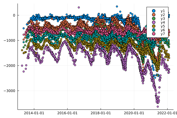
C = ItsLive.getvar(lat,lon,varnames, catalogdf)Plot a single variable for all points
ItsLive.plotvar(C,"vx")Plot a single point, single variable colored by sensor
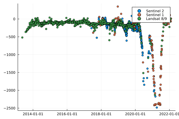
ItsLive.plotbysensor(C[1,:],"vx"); example_datacube_workflow.jl example script showing how to work with the ItsLive.jl package.
datacube_basic_pluto.jl A simple Pluto example that uses the ItsLive.jl package to retrieve and plot ITS_LIVE data.
catalogdf = ItsLive.catalog() return a DataFrame of the catalog for all of the ITS_LIVE zarr datacubes.
rownumdf = ItsLive.intersect(lat, lon, catalogdf) return the rownumber of the the DataFrame catalog (catalogdf) of the ITS_LIVE zarr datacubes that intersects the provided latitude and longitude.
x, y = ItsLive.nearestxy(lat, lon, DataArray) return the x/y indices into a ZarrGroup (DataArray) for the points nearest the provided latitude, longitude locations.
C = ItsLive.getvar(lat, lon, varnames, catalogdf) return a named m x n matrix of vectors with m = length(lat) rows and n = length(varnames)+2(for lat and lon) columns for the points nearest the lat/lon location from ITS_LIVE Zarr datacubes (catalogdf).
plotvar(C, varname)) plot ITS_LIVE data (C) variable (varname) for multiple points. Use keyword dtmax = Number to limit longer image-pair separations from being plotted.
plotbysensor(C, varname)) plot ITS_LIVE data (C) variable (varname) by sensor. Size(C,2) must = 1, e.g. C[1,:] of full matrix. Use keyword dtmax = Number to limit longer image-pair separations from being plotted.
binstats(x, y, [binedges = [0.0], dx= 0, method = "mean"]) return statistics of x central value and x spread according to method ["mean" = default] argument on values binned by y.
dtmax = dtfilter(x,dt) return the maximum dt for which the distribution of x show no statistical difference from the distribution of x in the minimum dt bin
This filter is needed to identify longer dts that exhibit "skipping" or "locking" behavior in feature tracking estimates of surface flow. This happens when the surface texture provides a lesser match than to stationary features, due to long time separation between repeat images, such as ice falls and curved medial moraines.
outlier, dtmax, sensorgroups = ItsLive.vxvyfilter(x,dt) applies dtfilter() to vx and vy projected on the their median vector and returns outlier BitVector, the maximum dt (dtmax) for which the distribution of vx or vy shows no statistical difference and the sensor groupings used when filtering the data (sensorgroups).
t_fit, v_fit, amp_fit, phase_fit, v_fit_err, amp_fit_err, fit_count, fit_outlier_frac, outlier = ItsLive.lsqfit_annual(v,v_err,mid_date,date_dt,mad_thresh) error wighted model fit to discrete interval data. The current model is an iterative fit to a sinusoidal function with unique mean (v_fit), phase (phase_fit) and amplitude (amp_fit) for each year of data centered at time t_fit. Errors are provided for annual means (v_fit_err) and amplitude (amp_fit_err). fit_count gives the number of velocity observations used for each year, fit_outlier_frac provides the fraction of data excluded from the model fit and a outlier BitVector.
v_i, v_i_err = ItsLive.lsqfit_interp(t_fit, v_fit, amp_fit, phase_fit, v_fit_err, amp_fit_err, t_i) evaluates the outputs of lsqfit at times t_i, outputting velocity (v_i) and velocity error (v_i_err) at times t_i.
v0 = ItsLive.running_mean(v, w) calculates the running mean of v with window size of w.
offset, slope, error = ItsLive.wliearfit(t, v, v_err, datetime0) returns the offset, slope, and error (error) for a weighted linear fit to v with a y-intercept of datetime0.
v, v,_err, dv_dt, v_amp, v_amp_err, v_phase = ItsLive.climatology_magnitude(vx0, vy0, vx0_err, vy0_err, dvx_dt, dvy_dt, vx_amp, vy_amp, vx_amp_err, vy_amp_err, vx_phase, vy_phase) returns the mean (v), standard error (v_err), trend (dv_dt), seasonal amplitude (v_amp), error in seasonal amplitude (v_amp_err), and seasonal phase (v_phase) from component values projected on the unit flow vector defined by vx0 and vy0.


