Deep learning is known to work well when applied to unstructured data like text, audio, or images but can sometimes lag behind other machine learning approaches like gradient boosting when applied to structured or tabular data. In this project, we will use semi-supervised learning to improve the performance of deep neural models when applied to structured data in a low data regime. We will show that by using unsupervised pre-training we can make a neural model perform better than gradient boosting.
This project is based on two papers:
- AutoInt: Automatic Feature Interaction Learning via Self-Attentive Neural Networks
- TabNet: Attentive Interpretable Tabular Learning
We implement a deep neural architecture that is similar to what is presented in the AutoInt paper, we use multi-head self-attention and feature embeddings. The pre-training part was taken from the Tabnet paper.
We will work on structured data, meaning data that can be written as a table with columns (numerical, categorical, ordinal) and rows. We also assume that we have a large number of unlabeled samples that we can use for pre-training and a small number of labeled samples that we can use for supervised learning. In the next experiments, we will simulate this setting to plot the learning curves and evaluate the approach when using different sizes of labeled sets.
Let’s use an example to describe how we prepare the data before feeding it to the neural network.
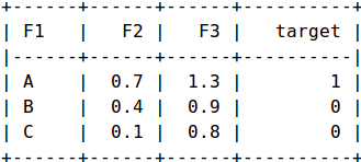
In this example, we have three samples and three features {F1, F2, F3}, and one target. F1 is a categorical feature while F2 and F3 are numeric features. We will create a new feature F1_X for each modality X of F1 and give it a value 1 if F1 == X else it is equal to 0.
The transformed samples will be written a set of (Feature_Name, Feature_Value).
For example:
First Sample -> {(F1_A, 1), (F2, 0.3), (F3,
1.3)}
Second Sample -> {(F1_B, 1), (F2, 0.4), (F3, 0.9)}
Third Sample -> {(F1_C, 1), (F2, 0.1), (F3, 0.8)}
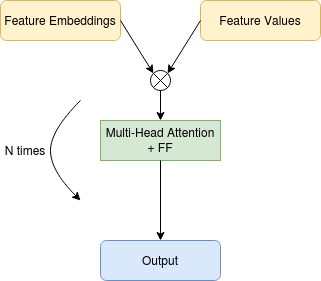
The feature names will be fed into an embedding layer and then will be multiplied with feature values.
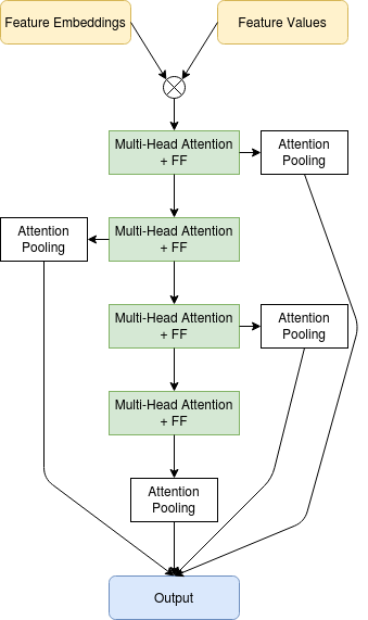
The model used here is a sequence of multi-head attention blocks and point-wise feed-forward layers. When training we also use Attention Pooled skip connections. The multi-head attention blocks allow us to model the interactions that might exist between the features while the Attention Pooled skip connections allow us to get a single vector from the set of feature embeddings.
Simplified Model — Image by author
Pre-training:
During the pre-training step we use the full unlabeled dataset and we input a corrupted version of the features and train the model to predict the uncorrupted features, similar to what you would do in a denoising auto-encoder.
Supervised Training:
During the supervised part of the training, we add skip connections between the encoder part and the output and we try to predict the target.
Simplified Model — Image by author
In the following experiments, we will use four datasets, two for regression and two for classification.
- Sarco: Has Around 50k samples, 21 features, and 7 continuous targets.
- Online News: Has Around 40k samples, 61 features, and 1 continuous target.
- Adult Census: Has Around 40k samples, 15 features, and 1 binary target.
- Forest Cover: Has Around 500k samples, 54 features, and 1 classification targets.
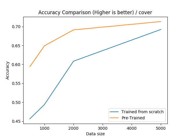
We will compare a pre-trained neural model to one that was trained from scratch, and we will focus on the performance on a low data regime, meaning a few hundred to a few thousand labeled samples. We will also do a comparison with a popular implementation of gradient boosting called lightgbm.
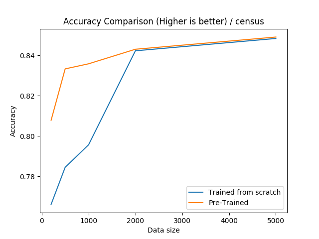
For this data-set, we can see that pre-training is very effective if the training set is smaller than 2000.
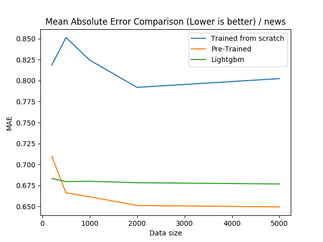
For the online news dataset, we can see that pre-training the neural networks are very effective, even over-performing gradient boosting for all sample sizes 500 and bigger.
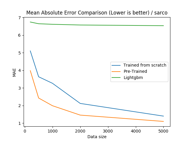
For the Sarco dataset, we can see that pre-training the neural networks are very effective, even over-performing gradient boosting for all sample sizes.
The code to reproduce the results is available here: https://github.com/CVxTz/DeepTabular
Using it you can easily train a classification or regression model->
import pandas as pd
from sklearn.model_selection import train_test_split

from deeptabular.deeptabular import DeepTabularClassifier

if __name__ == "__main__":
    data = pd.read_csv("../data/census/adult.csv")

    train, test = train_test_split(data, test_size=0.2, random_state=1337)

    target = "income"

    num_cols = ["age", "fnlwgt", "capital.gain", "capital.loss", "hours.per.week"]
    cat_cols = [
        "workclass",
        "education",
        "education.num",
        "marital.status",
        "occupation",
        "relationship",
        "race",
        "sex",
        "native.country",
    ]

    for k in num_cols:
        mean = train[k].mean()
        std = train[k].std()
        train[k] = (train[k] - mean) / std
        test[k] = (test[k] - mean) / std

    train[target] = train[target].map({"<=50K": 0, ">50K": 1})
    test[target] = test[target].map({"<=50K": 0, ">50K": 1})

    print(train[target].mean())

    classifier = DeepTabularClassifier(
        num_layers=10, cat_cols=cat_cols, num_cols=num_cols, n_targets=1,
    )

    classifier.fit(train, target_col=target, epochs=128)

    pred = classifier.predict(test)

    classifier.save_config("census_config.json")
    classifier.save_weigts("census_weights.h5")

    new_classifier = DeepTabularClassifier()

    new_classifier.load_config("census_config.json")
    new_classifier.load_weights("census_weights.h5")

    new_pred = new_classifier.predict(test)
Unsupervised pre-training is known to improve the performance of neural networks in the computer vision or natural language domain. In this project we demonstrate that it can also work when applied to structured data, making it competitive with other machine learning methods like gradient boosting in the low data regime.
Cite:
@software{mansar_youness_2020_4060165,
  author       = {Mansar Youness},
  title        = {CVxTz/DeepTabular: v1.0},
  month        = sep,
  year         = 2020,
  publisher    = {Zenodo},
  version      = {v1.0},
  doi          = {10.5281/zenodo.4060165},
  url          = {https://doi.org/10.5281/zenodo.4060165}
}
