The goal of clustRcompaR is to make it easy to cluster (or group) a series of documents (texts of any length), and to interpret these groups and to describe their frequency across factors, such as between different groups or over time.
You can install the development version of clustRcompaR from GitHub with:
# install.packages("devtools")
devtools::install_github("alishinski/clustRcompaR")
You can install the stable release on CRAN with:
install.packages("clustRcompaR")This is a basic example using the built-in inaugural addressess dataset.
First, we use cluster() to cluster the documents into three clusters. We include a new variable, year_before_1900, which we will later use to compare frequencies across clusters. Then we use extract_terms() to view the terms and term frequencies in the two clusters.
First, let's process the texts.
library(clustRcompaR)
library(dplyr)
#>
#> Attaching package: 'dplyr'
#> The following objects are masked from 'package:stats':
#>
#>     filter, lag
#> The following objects are masked from 'package:base':
#>
#>     intersect, setdiff, setequal, union

d <- inaugural_addresses
d <- mutate(d, century = ifelse(Year < 1800, "17th",
                                ifelse(Year >= 1800 & Year < 1900, "18th",
                                       ifelse(Year >= 1900 & Year < 2000, "19th", "20th"))))
Next, we cluster the texts.
three_clusters <- cluster(d, century, n_clusters = 3)
#> Document-feature matrix of: 58 documents, 2,820 features (79.6% sparse).
extract_terms(three_clusters)
#>    Cluster.1.Terms Cluster.1.Term.Frequencies Cluster.2.Terms
#> 1               in                  34.200000              in
#> 2               my                  13.866667           their
#> 3            their                  12.333333          govern
#> 4             will                  11.200000            will
#> 5           govern                   9.533333             has
#> 6            peopl                   7.200000              it
#> 7               it                   7.133333           state
#> 8           nation                   7.000000            been
#> 9              has                   6.733333           peopl
#> 10         countri                   6.533333          nation
#>    Cluster.2.Term.Frequencies Cluster.3.Terms Cluster.3.Term.Frequencies
#> 1                    77.52941              in                  36.692308
#> 2                    22.88235            will                  16.076923
#> 3                    21.41176          nation                  12.500000
#> 4                    20.29412              us                  12.038462
#> 5                    20.00000           world                   9.807692
#> 6                    19.41176           peopl                   9.307692
#> 7                    18.23529             can                   7.769231
#> 8                    17.82353            must                   7.730769
#> 9                    16.05882         america                   7.423077
#> 10                   14.41176              no                   7.192308
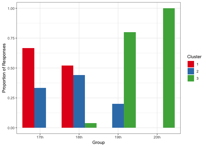
Then, we use the compare() function to compare the frequency of clusters across a factor, in this case, the century. We can then use the compare_plot() or compare_test() (which uses a Chi-Square test) function.
Here, we can compare the texts.
three_clusters_comparison <- compare(three_clusters, "century")
compare_plot(three_clusters_comparison)