Linseed (LINear Subspace identification for gene Expresion Deconvolution) is a package that provides tools and interface to explore gene expression datasets in linear space.
You can install the package using devtools::install_github:
devtools::install_github("ctlab/linseed")Current build was tested using rhub:
To start working with gene expression data, we need to create a new LinseedObject, in this tutorial we will use GSE19830 (mixture of Liver, Brain and Lung), we will take only mixed samples (10-42) and will take only 10000 most expressed genes.
library(linseed)
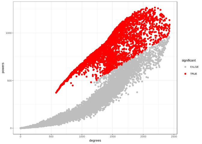
lo <- LinseedObject$new("GSE19830", samples=10:42, topGenes=10000)To build a coolinearity network we first have to evaluate all pairwise collinearity coefficients, all pairwise spearman correlation and then run significance test which will calculate p value for each each by shuffling network weights randomly.
lo$calculatePairwiseLinearity()
lo$calculateSpearmanCorrelation()
lo$calculateSignificanceLevel(100)
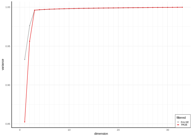
lo$significancePlot(0.01)lo$filterDatasetByPval(0.01)## Total number of genes is 10000
## The number of genes after filtering is 3297
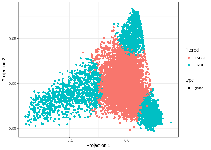
lo$svdPlot()To visualiaze what left after filtering we can call projection plot from our object. But we have to project the data to the simplex first.
lo$setCellTypeNumber(3)
lo$project("full") # projecting full dataset
lo$projectionPlot(color="filtered")To deconvolve the dataset, you first have to project (full or filtered dataset) to the simplex, and then find corners of it.
lo$project("filtered")
lo$smartSearchCorners(dataset="filtered", error="norm")
## Final vector is
## 4 1 5
##
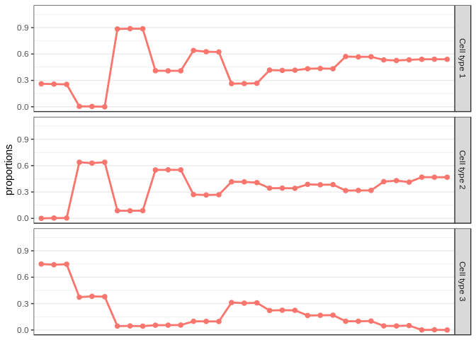
lo$deconvolveByEndpoints()
plotProportions(lo$proportions)
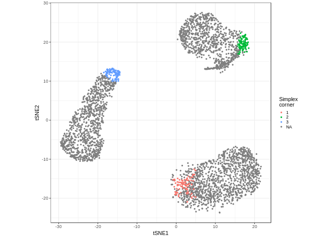
We can also use tSNE to haave an idea of how data looks like when dimensionally reduced.
# lets select 100 genes closest to the simplex corners
lo$selectGenes(100)
lo$tsnePlot()
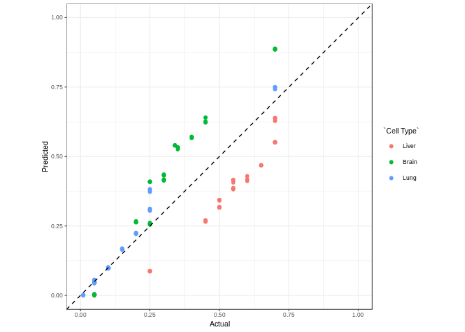
To compare with actual proportions you can use dotPlotProportions function
data("proportionsLiverBrainLung")
dotPlotPropotions(lo$proportions, proportionsLiverBrainLung[, 10:42], guess=TRUE)