This Code Pattern will guide you through how to use Scikit Learn and Python in IBM Watson Studio. The goal is to use a Jupyter notebook is to deep dive into Principal Component Analysis using the various dataset that are shipped with 'Scikit Learn'.
We will first give a short intuitive explanation for principal component analysis and why it makes sense. Then we will go deeper into the actual derivation of Principal Components using the principle of maximizing the total projected variances onto components. Once we have understood the theory and concept, we will dive deeper into the use cases and examples. We will consider four scenarios with examples.
- Dimension Reduction
- Visualization
- Noise Filtering
- As a pre-processor for ML algorithms.
In the end, we will summarize our discussion with various pointers to alternatives to PCA.
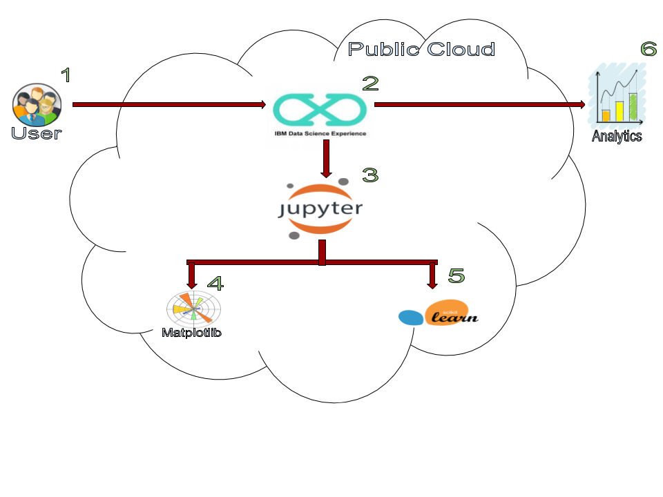
- Log into IBM Watson Studio service.
- Start a notebook in Watson Studio.
- Deep dive into intuitiona and theory of PCA.
- Consider four scenarios with Examples: 5.1. Dimension Reduction 5.2. Visualization 5.3. Noise Filtering 5.4. As a pre-processor for ML algorithms.
- IBM Watson Studio: Analyze data using RStudio, Jupyter, and Python in a configured, collaborative environment that includes IBM value-adds, such as managed Spark.
- Jupyter Notebook: An open source web application that allows you to create and share documents that contain live code, equations, visualizations, and explanatory text.
- Data Science: Systems and scientific methods to analyze structured and unstructured data in order to extract knowledge and insights.
- Python: Python is a programming language that lets you work more quickly and integrate your systems more effectively.
- Scikit Learn: A Python library for providing efficient tools for data mining and machine learning.
- Matplotlib: A Python library integrating matplot for visualization.
This Code Pattern consists of following activities:
- Sign up for the Watson Studio
- Create a new Watson Studio project
- Create the notebook
- Run the notebook
- Save and Share
Log in or sign up for IBM's Watson Studio.
Note: if you would prefer to skip the remaining Watson Studio set-up steps and just follow along by viewing the completed Notebook, simply:
- View the completed notebook and its outputs, as is.
- While viewing the notebook, you can optionally download it to store for future use.
- When complete, continue this code pattern by jumping ahead to the Principal Component Analysis in Practice. section.
- Select the
New Projectoption from the Watson Studio landing page and choose theData Scienceoption.
- To create a project in Watson Studio, give the project a name and either create a new
Cloud Object Storageservice or select an existing one from your IBM Cloud account.
- Upon a successful project creation, you are taken to a dashboard view of your project. Take note of the
AssetsandSettingstabs, we'll be using them to associate our project with any external assets (datasets and notebooks) and any IBM cloud services.
- From the project dashboard view, click the
Assetstab, click the+ New notebookbutton.
-
Give your notebook a name and select your desired runtime, in this case we'll be using python Runtime.
-
Now select the
From URLtab to specify the URL to the notebook in this repository.
- Enter this URL:
https://github.com/aloknsingh/ds_pca_deep_dive/blob/master/notebooks/deep_dive_pca.ipynb
- Click the
Createbutton.
Note: If queried for a Python version, select version
3.5.
When a notebook is executed, what is actually happening is that each code cell in the notebook is executed, in order, from top to bottom.
Each code cell is selectable and is preceded by a tag in the left margin. The tag
format is In [x]:. Depending on the state of the notebook, the x can be:
- A blank, this indicates that the cell has never been executed.
- A number, this number represents the relative order this code step was executed.
- A
*, this indicates that the cell is currently executing.
There are several ways to execute the code cells in your notebook:
- One cell at a time.
- Select the cell, and then press the
Playbutton in the toolbar.
- Select the cell, and then press the
- Batch mode, in sequential order.
- From the
Cellmenu bar, there are several options available. For example, you canRun Allcells in your notebook, or you canRun All Below, that will start executing from the first cell under the currently selected cell, and then continue executing all cells that follow.
- From the
- At a scheduled time.
- Press the
Schedulebutton located in the top right section of your notebook panel. Here you can schedule your notebook to be executed once at some future time, or repeatedly at your specified interval.
- Press the
Under the File menu, there are several ways to save your notebook:
Savewill simply save the current state of your notebook, without any version information.Save Versionwill save your current state of your notebook with a version tag that contains a date and time stamp. Up to 10 versions of your notebook can be saved, each one retrievable by selecting theRevert To Versionmenu item.
You can share your notebook by selecting the Share button located in the top
right section of your notebook panel. The end result of this action will be a URL
link that will display a “read-only” version of your notebook. You have several
options to specify exactly what you want shared from your notebook:
Only text and output: will remove all code cells from the notebook view.All content excluding sensitive code cells: will remove any code cells that contain a sensitive tag. For example,# @hidden_cellis used to protect your credentials from being shared.All content, including code: displays the notebook as is.- A variety of
download asoptions are also available in the menu.
Through various real life examples, we give user intuition of PCA.
We give user mathemathical foundation and derive the key idea of PCA.
Once, We have seen, intuition and mathematical formulation of Principal Component Analysis. We explore PCA through various examples. We will be using Scikit-learn and matplotlib to dive deep into examples.
We will look into following four use cases:
-
PCA for Dimension Reduction.
-
PCA for Visualization and Better Insights.
-
PCA for Noise Filtering.
-
PCA as a Preprocessor for ML algorithms.
The following screen-shot shows, derivation of PCA by maximizing total projected variances.

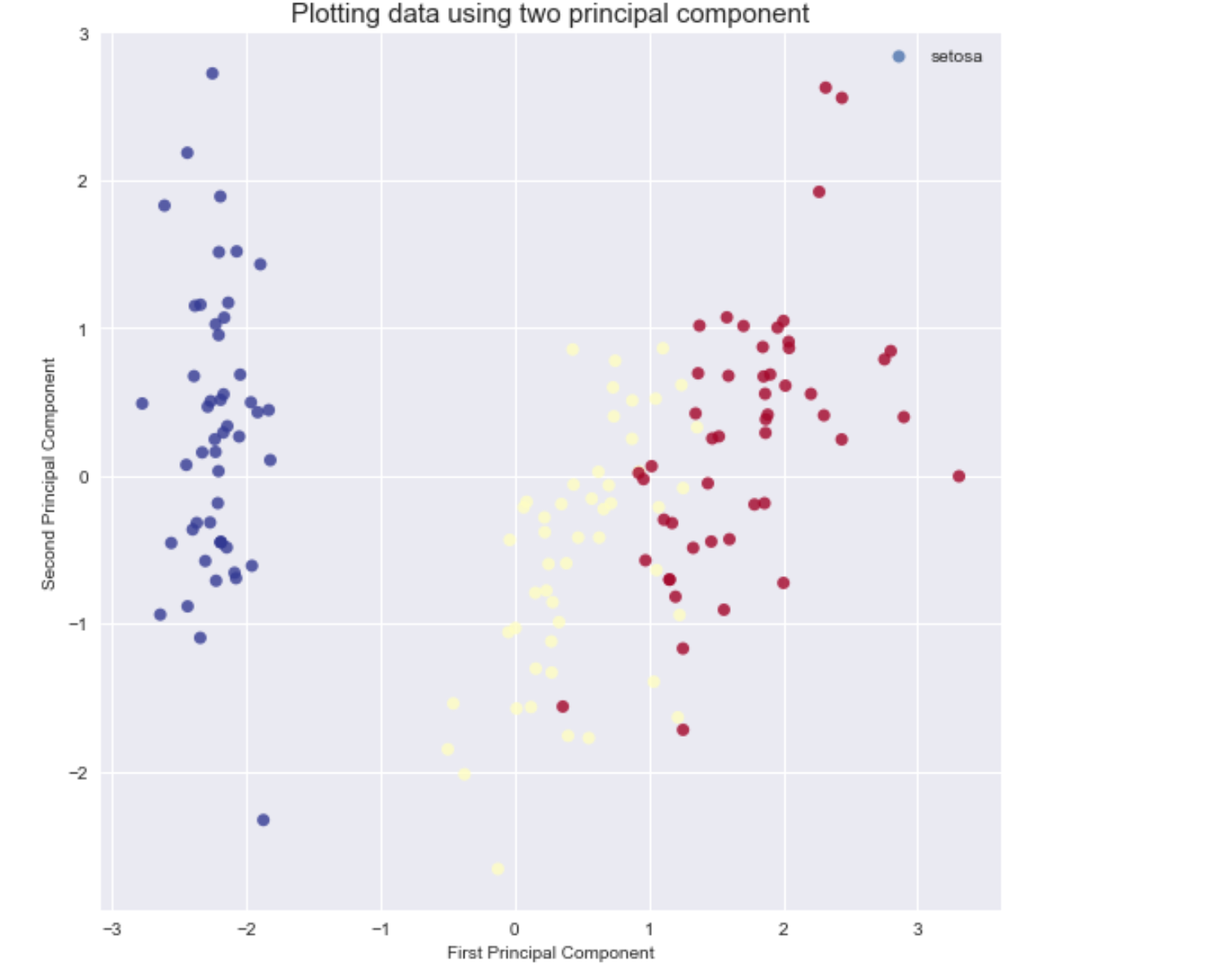
The following screen-shot shows, how one can do simple classification using PCA.

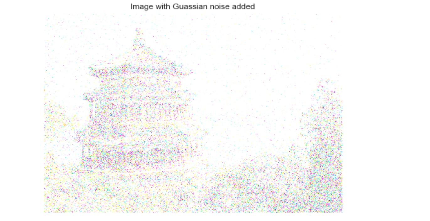
The following screen-shots show, how to de-noise a noisy image using PCA.


Awesome job following along! Now go try and take this further or apply it to a different use case!
- Watson Studio: https://datascience.ibm.com/docs/content/analyze-data/creating-notebooks.html.
- Scikit Learn: http://scikit-learn.org/stable/
- Matplotlib: https://matplotlib.org/
- SeaBorn: https://seaborn.pydata.org
- Data Analytics Code Patterns: Enjoyed this Code Pattern? Check out our other Data Analytics Code Patterns
- AI and Data Code Pattern Playlist: Bookmark our playlist with all of our Code Pattern videos
- Data Science Experience: Master the art of data science with IBM's Data Science Experience


