The ggh4x package provides some utility functions that are don’t entirely fit within the ‘grammar of graphics’ concept —they can be a bit hacky— but can nonetheless be useful in tweaking your ggplots. Examples include adjusting the sizes of facets, mapping multiple aesthetics to colours and specififying individual scales for facets. Besides this, it is also a small collection of geoms, facets, positions and stats.
You can install the development version from GitHub with:
# install.packages("devtools")
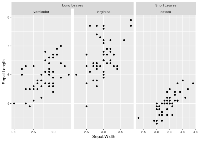
devtools::install_github("teunbrand/ggh4x")This example illustrates how you can use nested facets:
library(ggh4x)
#> Loading required package: ggplot2

df <- iris
df$Nester <- ifelse(df$Species == "setosa", "Short Leaves", "Long Leaves")

g <- ggplot(df, aes(Sepal.Width, Sepal.Length)) +
  facet_nested(~ Nester + Species, scales = "free")

g + geom_point()
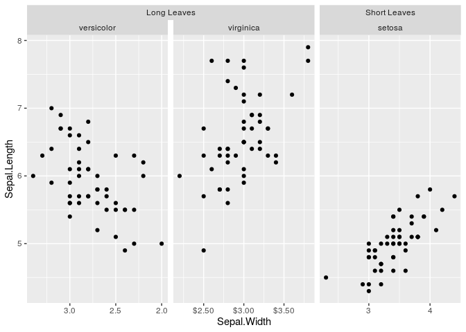
Sometimes, you might want to vary the scales of your facets
independently from oneanother. You could use facetted_pos_scales() to
achieve this, and the facet argument scales had to be set to free.
scales <- list(
  scale_x_reverse(),
  scale_x_continuous(labels = scales::dollar),
  scale_x_continuous(breaks = c(3, 4))
)

g <- g + facetted_pos_scales(x = scales)
g + geom_point()
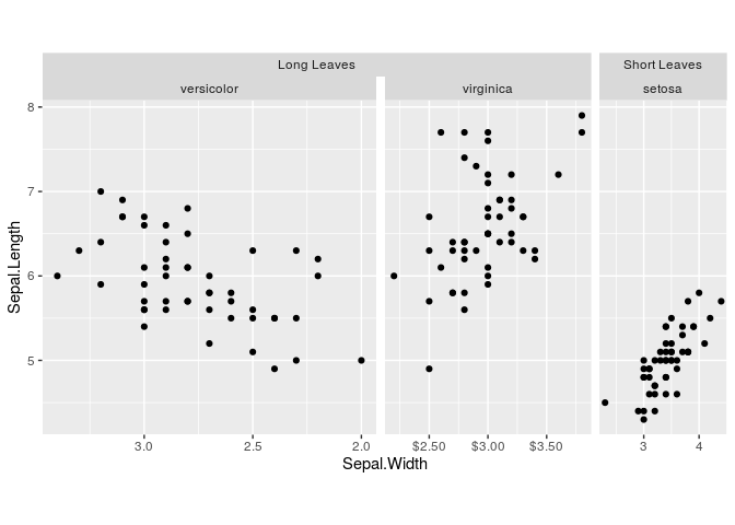
If you don’t like the sizes of the facet panels, you can tweak these
using force_panelsizes() in a data-independent manner, without having
to rely on facet_grid’s space = "free" argument.
# Inverse golden ratio
phi <- 2 / (1 + sqrt(5))

g <- g + force_panelsizes(rows = 1, cols = c(1, phi, phi^2), respect = TRUE)

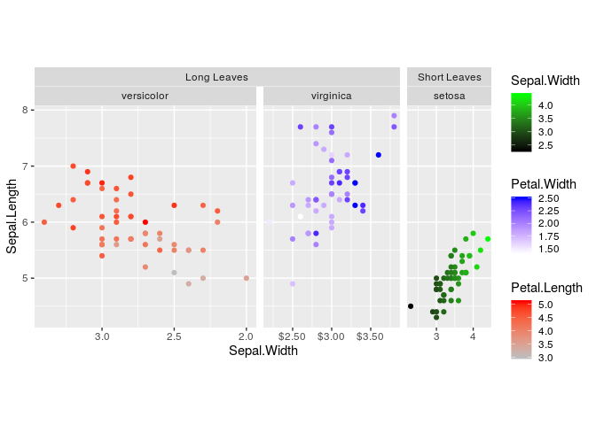
g + geom_point()One colourscale is in some cases not sufficient to describe your data.
You can map several variables to colours with scale_colour_multi() if
data are in seperate layers. You can see from all the warnings that some
functions in this package might be called ‘hacks’.
# ggsubset is a convenience function to pull data from
# the main ggplot call in layers
g <- g +
  geom_point(aes(swidth = Sepal.Width),
             ggsubset(Species == "setosa")) +
  geom_point(aes(pleng  = Petal.Length),
             ggsubset(Species == "versicolor")) +
  geom_point(aes(pwidth = Petal.Width),
             ggsubset(Species == "virginica"))
#> Warning: Ignoring unknown aesthetics: swidth
#> Warning: Ignoring unknown aesthetics: pleng
#> Warning: Ignoring unknown aesthetics: pwidth

g <- g + scale_colour_multi(
  aesthetics = c("swidth", "pleng", "pwidth"),
  colours = list(c("black", "green"),
                 c("gray", "red"),
                 c("white", "blue")),
  guide = guide_colourbar(barheight = unit(50, "pt"))
)
g
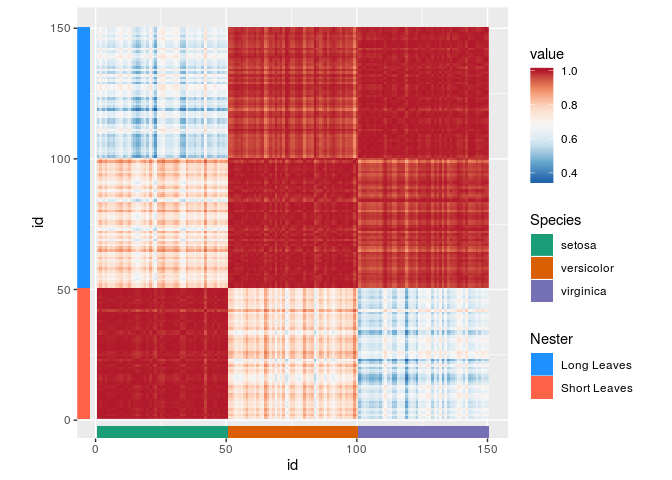
Mixing continuous and discrete colours can also be done, with the
slightly more verbose scale_listed(), such as in the following
heatmap.
# Making an iris correlation-heatmap
iriscor <- cor(t(iris[, 1:4]))
iriscor <- data.frame(
  x = as.vector(row(iriscor)),
  y = as.vector(col(iriscor)),
  value = as.vector(iriscor)
)

df$id <- seq_len(nrow(df))


# Setting up a basic heatmap
g <- ggplot(df, aes(id, id)) +
  # geom_tilemargin can be useful for annotating heatmaps
  geom_tilemargin(aes(species = Species),
                  sides = "b") +
  geom_tilemargin(aes(leave = Nester),
                  sides = "l") +
  geom_raster(aes(x, y, cor = value),
              data = iriscor) +
  coord_fixed()
#> Warning: Ignoring unknown aesthetics: species
#> Warning: Ignoring unknown aesthetics: leave
#> Warning: Ignoring unknown aesthetics: cor

# Adding the colour scales
g <- g + scale_listed(scalelist = list(
  scale_fill_distiller(palette = "RdBu", aesthetics = "cor"),
  scale_fill_brewer(palette = "Dark2", aesthetics = "species"),
  scale_fill_manual(values = c("dodgerblue", "tomato"),
                    aesthetics = "leave")
), replaces = rep("fill", 3))
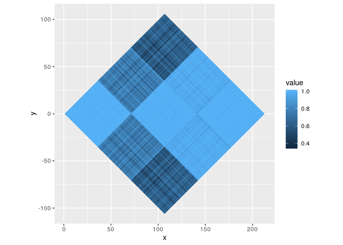
gOn the topic of rasters, if parameterised as a polygon with
geom_polygonraster(), they can subjected to linear transformations
such as rotations and shears with position_lineartrans().
g <- ggplot(iriscor, aes(x, y, fill = value)) +
  geom_polygonraster(position = position_lineartrans(angle = 45))

g + coord_fixed()
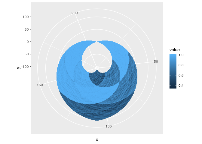
In fact, you could even do non-linear transformation with polygon-rasters, should you dare venture that way.
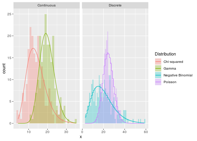
g + coord_polar()Ever get tired of unparameterised kernel density estimates? Now you can
fit a wide range of theoretical densities from the fitdistrplus
package to your data on the fly!
set.seed(1)
n <- 200
df <- data.frame(
  x = c(rpois(n, 25), rnbinom(n, 5, 0.2),
        rgamma(n, 30, 1.5), rchisq(n, 15)),
  class = rep(c("Discrete", "Continuous"), each = n*2),
  Distribution = rep(c("Poisson", "Negative Binomial",
                       "Gamma", "Chi-squared"),
                     each = n)
)

ggplot(df, aes(x, fill = Distribution, colour = Distribution)) +
  geom_histogram(position = "identity", binwidth = 1,
                 alpha = 0.3, colour = NA) +
  stat_theodensity(aes(y = stat(count)),
                   ggsubset(class == "Discrete"),
                   distri = "nbinom", geom = "step",
                   position = position_nudge(x = -0.5)) +
  stat_theodensity(aes(y = stat(count)),
                   ggsubset(class == "Continuous"),
                   distri = "gamma") +
facet_grid(~ class, scales = "free_x")I would like to mention that there are also packages that do some similar things to what this package does. facetscales also has a facet function wherein scales can set per row/colum. The relayer and ggnewscale packages also allow multiple colour scales in the same plot.
Historically, many of these functions come from the ggnomics package, but have been moved here as a package independent of Bioconductor infrastructure.

