This repo contains the full Jupyter Notebook and code for the Python talk on machine learning explainabilty and algorithmic bias.
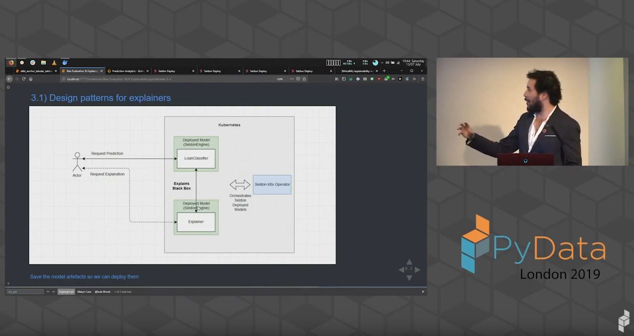
| This Video of talk presented at PyData London 2019 which provides an overview on the motivations for machine learning explainability as well as techniques to introduce explainability and mitigate undesired biases. |
|
| The presentation was performed using the RISE plugin to convert the Jupyter notebook into a reveal.js presentation. The reveal.js presentation is hosted live in this repo under the index.html page. |
|
Code examples to try it yourself:
- Data analysis for data imbalances with XAI
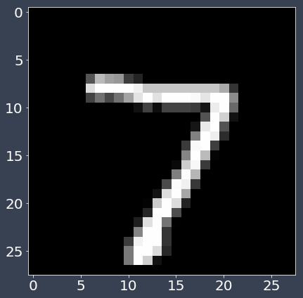
- Black box model evaluation for MNISt with Alibi
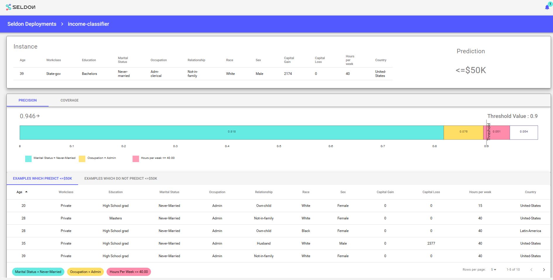
- Production monitoring with Seldon and Alibi
This example uses the following open source libraries:
- XAI - We use XAI to showcase data analysis techniques
- Alibi - We use Alibi to dive into black box model evaluation techniques
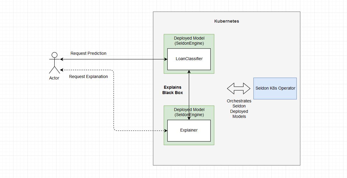
- Seldon Core - We use seldon core to deploy and serve ML models and ML explainers
In this next section below you can find the sumarised version of Jupyter notebook / presentation slides in Markdown format.
This section below contains the code blocks that summarise the 3 steps proposed in the presentation proposed for explainability: 1) Data analysis, 2) Model evaluation and 3) Production monitoring.
1.1) Data imbalances
1.2) Upsampling / downsampling
1.3) Correlations
1.4) Train / test set
1.5) Further techniques
We'll be using the XAI library which is a set of tools to explain machine learning data
X, y, X_train, X_valid, y_train, y_valid, X_display, y_display, df, df_display \
    = get_dataset_2()
df_display.head().dataframe tbody tr th {
vertical-align: top;
}
.dataframe thead th {
text-align: right;
}
| age | workclass | education | education-num | marital-status | occupation | relationship | ethnicity | gender | capital-gain | capital-loss | hours-per-week | native-country | loan | |
|---|---|---|---|---|---|---|---|---|---|---|---|---|---|---|
| 0 | 39 | State-gov | Bachelors | 13 | Never-married | Adm-clerical | Not-in-family | White | Male | 2174 | 0 | 40 | United-States | False |
| 1 | 50 | Self-emp-not-inc | Bachelors | 13 | Married-civ-spouse | Exec-managerial | Husband | White | Male | 0 | 0 | 13 | United-States | False |
| 2 | 38 | Private | HS-grad | 9 | Divorced | Handlers-cleaners | Not-in-family | White | Male | 0 | 0 | 40 | United-States | False |
| 3 | 53 | Private | 11th | 7 | Married-civ-spouse | Handlers-cleaners | Husband | Black | Male | 0 | 0 | 40 | United-States | False |
| 4 | 28 | Private | Bachelors | 13 | Married-civ-spouse | Prof-specialty | Wife | Black | Female | 0 | 0 | 40 | Cuba | False |
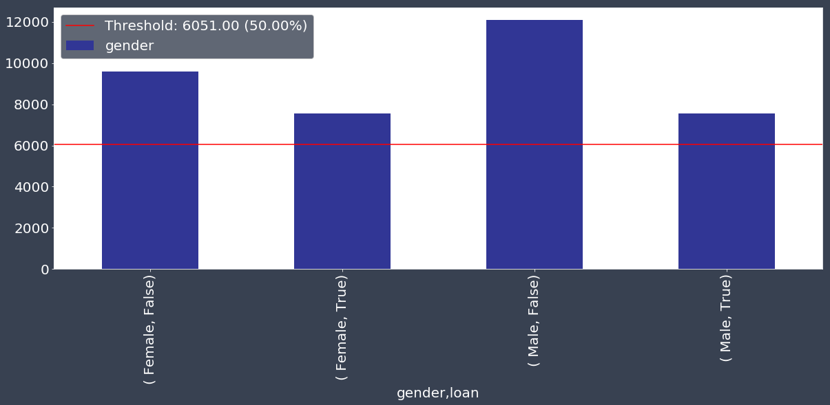
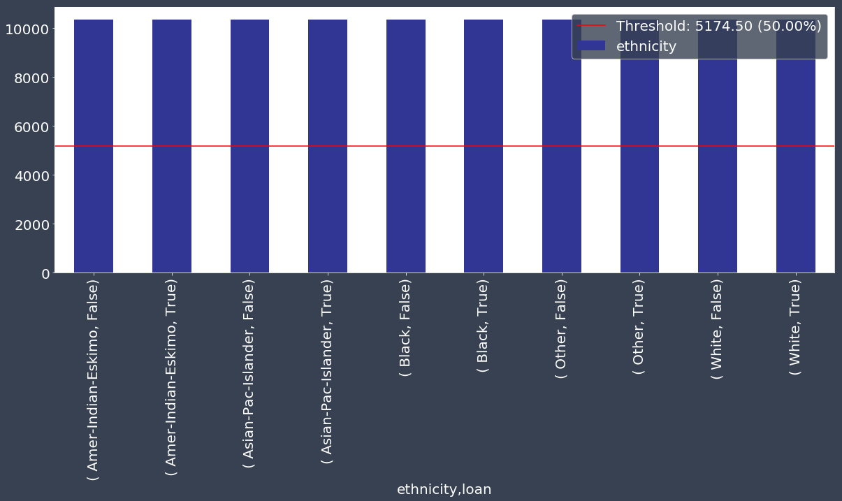
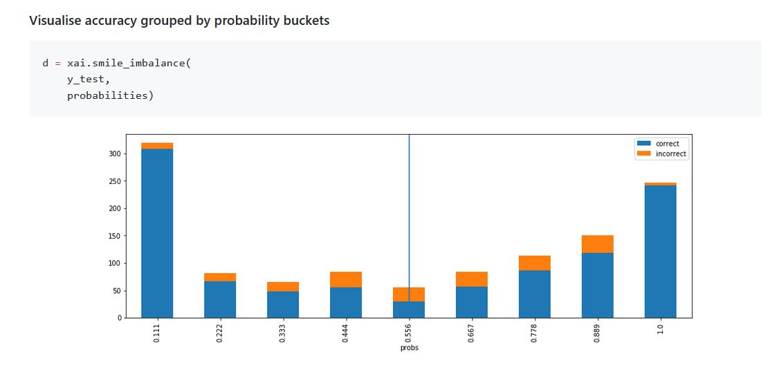
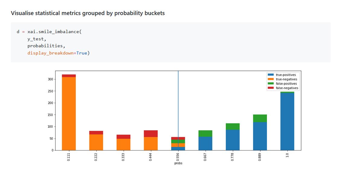
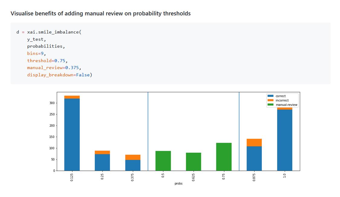
im = xai.imbalance_plot(df_display, "gender", threshold=0.55, categorical_cols=["gender"])im = xai.imbalance_plot(df_display, "gender", "loan" , categorical_cols=["loan", "gender"])im = xai.imbalance_plot(df_display, "age" , bins=10)im = xai.balance(df_display, "ethnicity", "loan", categorical_cols=["ethnicity", "loan"],
upsample=0.5, downsample=0.5, bins=5)1.3 Correlations hidden in data
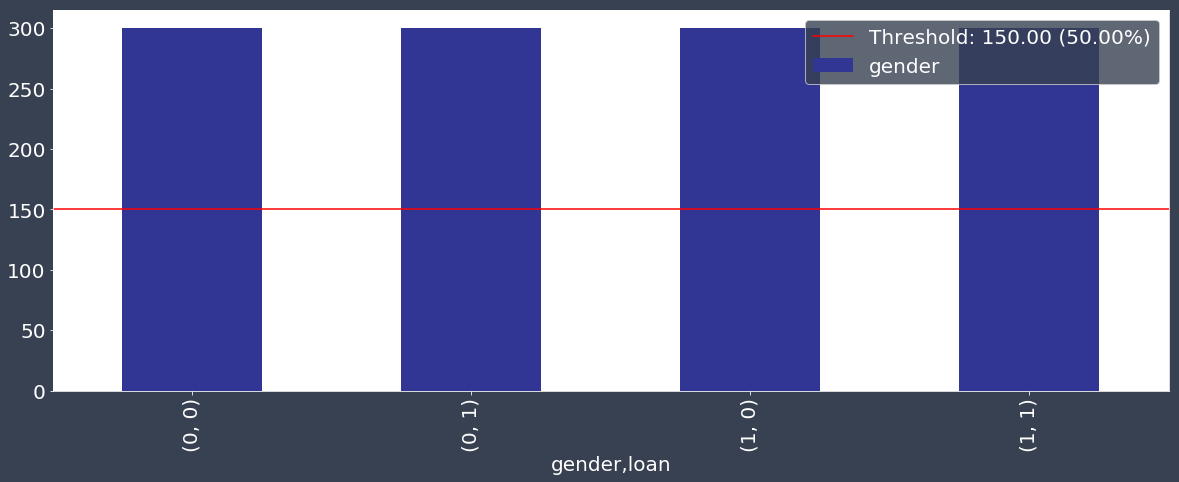
corr = xai.correlations(df_display, include_categorical=True)X_train_balanced, y_train_balanced, X_valid_balanced, y_valid_balanced, train_idx, test_idx = \
xai.balanced_train_test_split(
X, y, "gender",
min_per_group=300,
max_per_group=300,
categorical_cols=["gender", "loan"])
X_valid_balanced["loan"] = y_valid_balanced
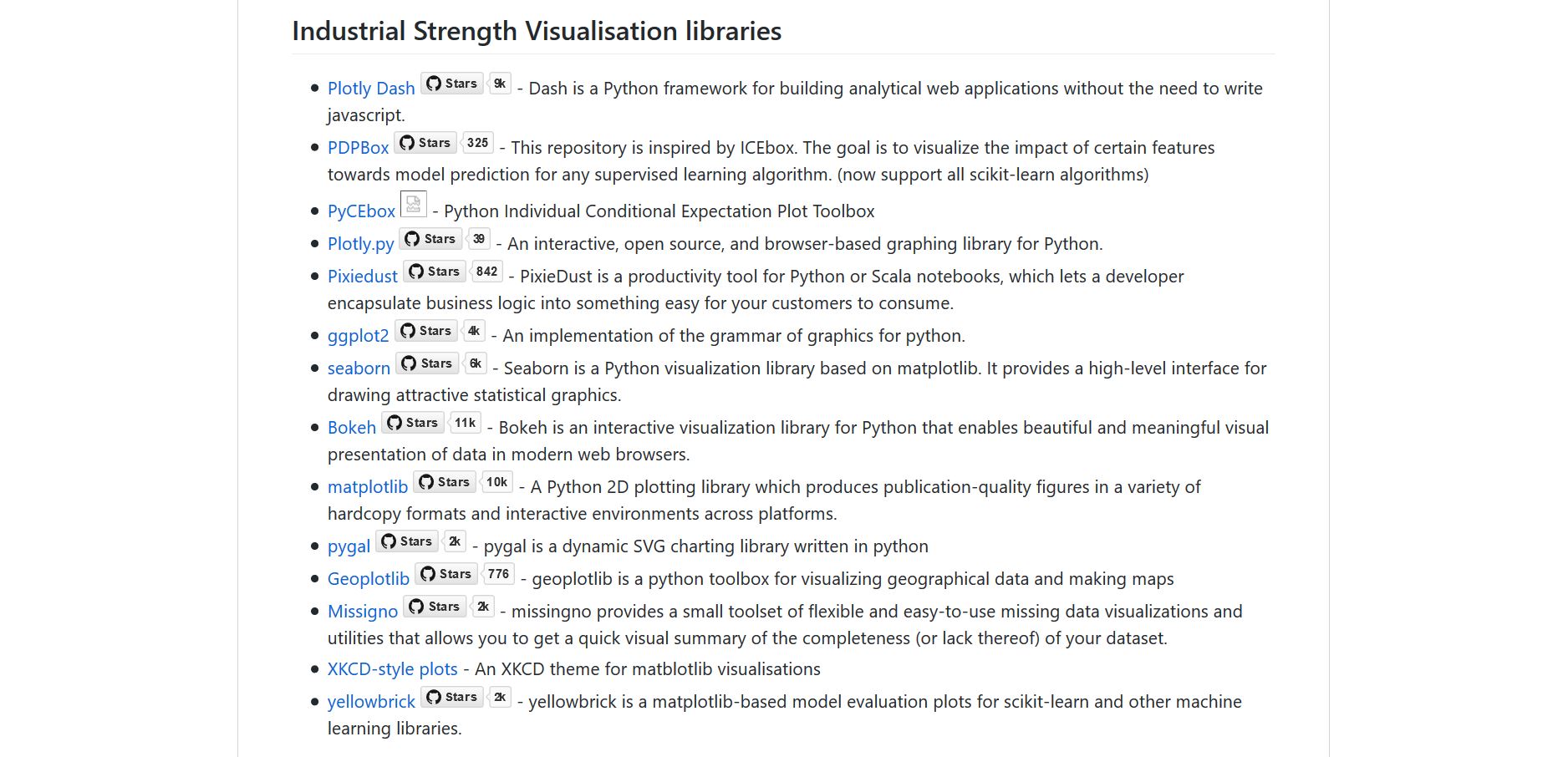
im = xai.imbalance_plot(X_valid_balanced, "gender", "loan", categorical_cols=["gender", "loan"])https://github.com/EthicalML/awesome-production-machine-learning#industrial-strength-visualisation-libraries
2.1) Standard model evaluation metrics
2.2) Global model explanation techniques
2.3) Black box local model explanation techniques
2.4) Other libraries available
# Let's start by building our model with our newly balanced dataset
model = build_model(X)
model.fit(f_in(X_train), y_train, epochs=20, batch_size=512, shuffle=True, validation_data=(f_in(X_valid), y_valid), callbacks=[PlotLossesKeras()], verbose=0, validation_split=0.05,)
probabilities = model.predict(f_in(X_valid))
pred = f_out(probabilities)
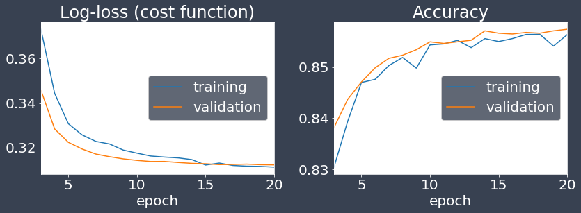
Log-loss (cost function):
training (min: 0.311, max: 0.581, cur: 0.311)
validation (min: 0.312, max: 0.464, cur: 0.312)
Accuracy:
training (min: 0.724, max: 0.856, cur: 0.856)
validation (min: 0.808, max: 0.857, cur: 0.857)
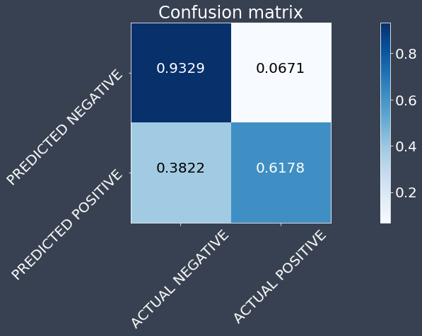
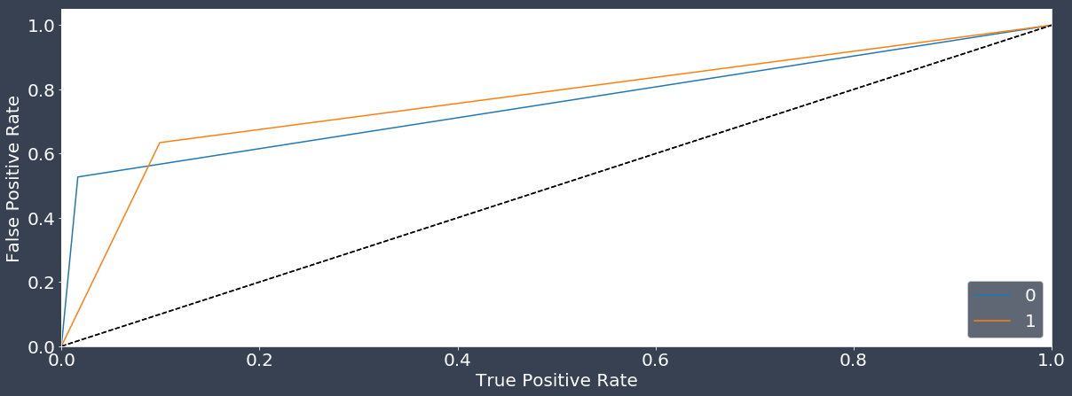
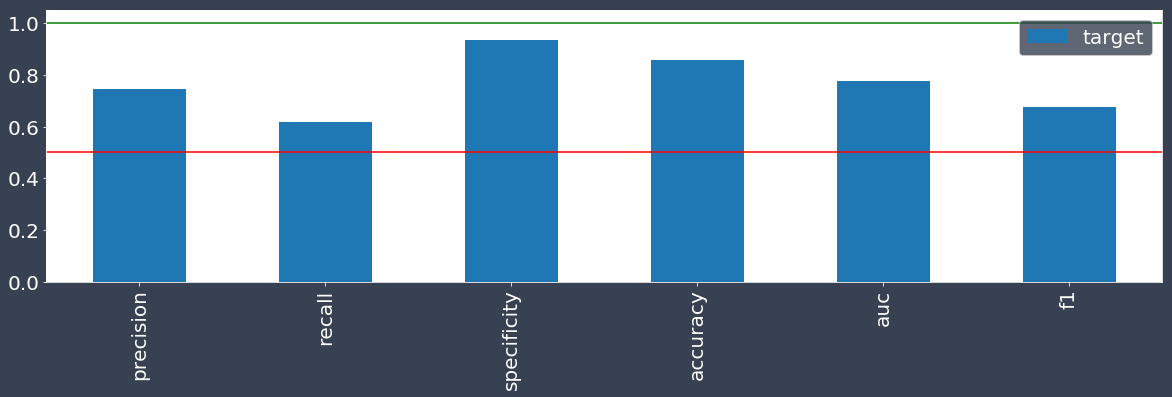
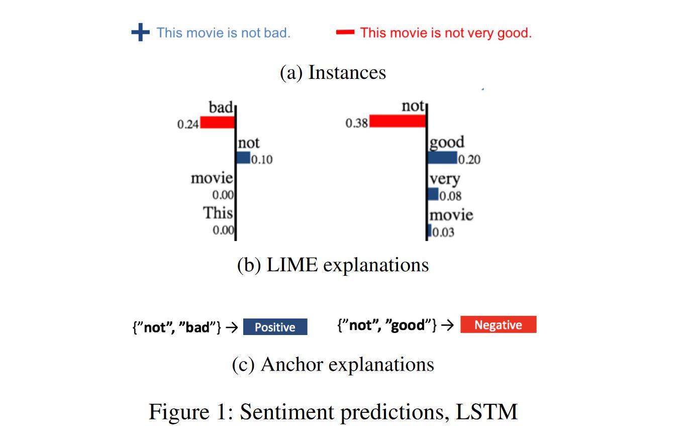
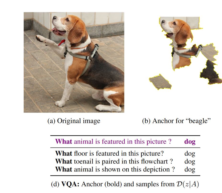
xai.confusion_matrix_plot(y_valid, pred)im = xai.roc_plot(y_valid, pred)im = xai.roc_plot(y_valid, pred, df=X_valid, cross_cols=["gender"], categorical_cols=["gender"])im = xai.metrics_plot(y_valid, pred)im = xai.metrics_plot(y_valid, pred, df=X_valid, cross_cols=["gender"], categorical_cols="gender")imp = xai.feature_importance(X_valid, y_valid, lambda x, y: model.evaluate(f_in(x), y, verbose=0)[1], repeat=1)Consists of if-then rules, called the anchors, which sufficiently guarantee the explanation locally and try to maximize the area for which the explanation holds. (ArXiv: Anchors: High-Precision Model-Agnostic Explanations)
from alibi.explainers import AnchorTabular

explainer = AnchorTabular(
    loan_model_alibi.predict,
    feature_names_alibi,
    categorical_names=category_map_alibi)

explainer.fit(
    X_train_alibi,
    disc_perc=[25, 50, 75])

print("Explainer built")
Explainer built
X_test_alibi[:1]array([[52, 4, 0, 2, 8, 4, 2, 0, 0, 0, 60, 9]])
explanation = explainer.explain(X_test_alibi[:1], threshold=0.95)

print('Anchor: %s' % (' AND '.join(explanation['names'])))
print('Precision: %.2f' % explanation['precision'])
print('Coverage: %.2f' % explanation['coverage'])
Anchor: Marital Status = Separated AND Sex = Female AND Capital Gain <= 0.00
Precision: 0.97
Coverage: 0.10
The counterfactual explanation of an outcome or a situation Y takes the form “If X had not occured, Y would not have occured”
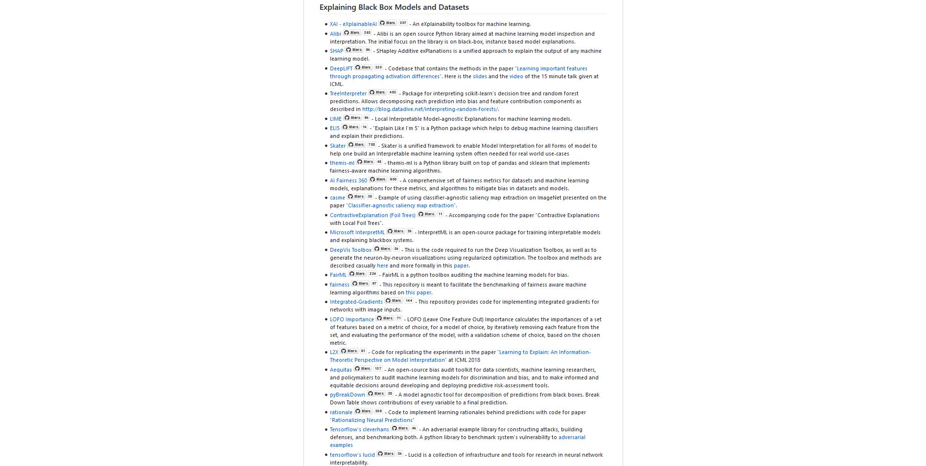
https://github.com/EthicalML/awesome-production-machine-learning#explaining-black-box-models-and-datasets
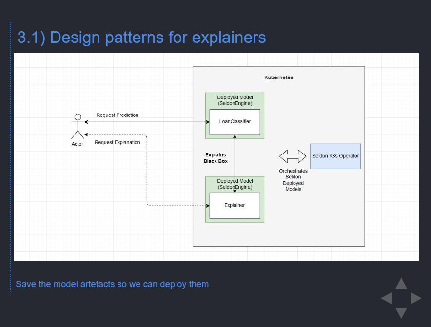
- Design patterns for explainers
- Live demo of explainers
- Leveraging humans for explainers
%%bash
kubectl create clusterrolebinding kube-system-cluster-admin --clusterrole=cluster-admin --serviceaccount=kube-system:default
helm init
kubectl rollout status deploy/tiller-deploy -n kube-system
helm install seldon-core-operator --name seldon-core-operator --repo https://storage.googleapis.com/seldon-charts
helm install seldon-core-analytics --name seldon-core-analytics --repo https://storage.googleapis.com/seldon-charts
helm install stable/ambassador --name ambassador
from sklearn.preprocessing import LabelEncoder, StandardScaler, OneHotEncoder
from sklearn.impute import SimpleImputer
from sklearn.pipeline import Pipeline
from sklearn.compose import ColumnTransformer
# feature transformation pipeline
ordinal_features = [x for x in range(len(alibi_feature_names)) if x not in list(alibi_category_map.keys())]
ordinal_transformer = Pipeline(steps=[('imputer', SimpleImputer(strategy='median')),
('scaler', StandardScaler())])
categorical_features = list(alibi_category_map.keys())
categorical_transformer = Pipeline(steps=[('imputer', SimpleImputer(strategy='median')),
('onehot', OneHotEncoder(handle_unknown='ignore'))])
preprocessor = ColumnTransformer(transformers=[('num', ordinal_transformer, ordinal_features),
('cat', categorical_transformer, categorical_features)])preprocessor.fit(alibi_data)from sklearn.ensemble import RandomForestClassifier
np.random.seed(0)
clf = RandomForestClassifier(n_estimators=50)
clf.fit(preprocessor.transform(X_train_alibi), y_train_alibi)!mkdir -p pipeline/pipeline_steps/loanclassifier/import dill
with open("pipeline/pipeline_steps/loanclassifier/preprocessor.dill", "wb") as prep_f:
dill.dump(preprocessor, prep_f)
with open("pipeline/pipeline_steps/loanclassifier/model.dill", "wb") as model_f:
dill.dump(clf, model_f)%%writefile pipeline/pipeline_steps/loanclassifier/Model.py
import dill
class Model:
def __init__(self, *args, **kwargs):
with open("preprocessor.dill", "rb") as prep_f:
self.preprocessor = dill.load(prep_f)
with open("model.dill", "rb") as model_f:
self.clf = dill.load(model_f)
def predict(self, X, feature_names=[]):
X_prep = self.preprocessor.transform(X)
proba = self.clf.predict_proba(X_prep)
return proba%%writefile pipeline/pipeline_steps/loanclassifier/requirements.txt
scikit-learn==0.20.1
dill==0.2.9
scikit-image==0.15.0
scikit-learn==0.20.1
scipy==1.1.0
numpy==1.15.4!mkdir pipeline/pipeline_steps/loanclassifier/.s2i%%writefile pipeline/pipeline_steps/loanclassifier/.s2i/environment
MODEL_NAME=Model
API_TYPE=REST
SERVICE_TYPE=MODEL
PERSISTENCE=0!s2i build pipeline/pipeline_steps/loanclassifier seldonio/seldon-core-s2i-python3:0.8 loanclassifier:0.1%%writefile pipeline/pipeline_steps/loanclassifier/loanclassifiermodel.yaml
apiVersion: machinelearning.seldon.io/v1alpha2
kind: SeldonDeployment
metadata:
labels:
app: seldon
name: loanclassifier
spec:
name: loanclassifier
predictors:
- componentSpecs:
- spec:
containers:
- image: loanclassifier:0.1
name: model
graph:
children: []
name: model
type: MODEL
endpoint:
type: REST
name: loanclassifier
replicas: 1!kubectl apply -f pipeline/pipeline_steps/loanclassifier/loanclassifiermodel.yamlX_test_alibi[:1]array([[52, 4, 0, 2, 8, 4, 2, 0, 0, 0, 60, 9]])
%%bash
curl -X POST -H 'Content-Type: application/json' \
    -d "{'data': {'names': ['text'], 'ndarray': [[52,  4,  0,  2,  8,  4,  2,  0,  0,  0, 60,  9]]}}" \
    http://localhost:80/seldon/default/loanclassifier/api/v0.1/predictions
{
"meta": {
"puid": "96cmdkc4k1c6oassvpnpasqbgf",
"tags": {
},
"routing": {
},
"requestPath": {
"model": "loanclassifier:0.1"
},
"metrics": []
},
"data": {
"names": ["t:0", "t:1"],
"ndarray": [[0.86, 0.14]]
}
}
% Total % Received % Xferd Average Speed Time Time Time Current
Dload Upload Total Spent Left Speed
100 356 100 264 100 92 11000 3833 --:--:-- --:--:-- --:--:-- 15478
from seldon_core.seldon_client import SeldonClient

batch = X_test_alibi[:1]

sc = SeldonClient(
    gateway="ambassador",
    gateway_endpoint="localhost:80",
    deployment_name="loanclassifier",
    payload_type="ndarray",
    namespace="default",
    transport="rest")

client_prediction = sc.predict(data=batch)

print(client_prediction.response)
meta {
puid: "hv4dnmr8m3ckgrhtnc48rs7mjg"
requestPath {
key: "model"
value: "loanclassifier:0.1"
}
}
data {
names: "t:0"
names: "t:1"
ndarray {
values {
list_value {
values {
number_value: 0.86
}
values {
number_value: 0.14
}
}
}
}
}
from alibi.explainers import AnchorTabular

predict_fn = lambda x: clf.predict(preprocessor.transform(x))
explainer = AnchorTabular(predict_fn, alibi_feature_names, categorical_names=alibi_category_map)
explainer.fit(X_train_alibi, disc_perc=[25, 50, 75])

explanation = explainer.explain(X_test_alibi[0], threshold=0.95)

print('Anchor: %s' % (' AND '.join(explanation['names'])))
print('Precision: %.2f' % explanation['precision'])
print('Coverage: %.2f' % explanation['coverage'])
Anchor: Marital Status = Separated AND Sex = Female AND Capital Gain <= 0.00
Precision: 0.97
Coverage: 0.10
def predict_remote_fn(X):
    from seldon_core.seldon_client import SeldonClient
    from seldon_core.utils import get_data_from_proto

    kwargs = {
        "gateway": "ambassador",
        "deployment_name": "loanclassifier",
        "payload_type": "ndarray",
        "namespace": "default",
        "transport": "rest"
    }

    try:
        kwargs["gateway_endpoint"] = "localhost:80"
        sc = SeldonClient(**kwargs)
        prediction = sc.predict(data=X)
    except:
        # If we are inside the container, we need to reach the ambassador service directly
        kwargs["gateway_endpoint"] = "ambassador:80"
        sc = SeldonClient(**kwargs)
        prediction = sc.predict(data=X)

    y = get_data_from_proto(prediction.response)
return y# Summary of the predict_remote_fn
def predict_remote_fn(X):
....
sc = SeldonClient(...)
prediction = sc.predict(data=X)
y = get_data_from_proto(prediction.response)
return yfrom seldon_core.utils import get_data_from_proto
explainer = AnchorTabular(predict_remote_fn, alibi_feature_names, categorical_names=alibi_category_map)
explainer.fit(X_train_alibi, disc_perc=[25, 50, 75])
explanation = explainer.explain(X_test_alibi[idx], threshold=0.95)
print('Anchor: %s' % (' AND '.join(explanation['names'])))
print('Precision: %.2f' % explanation['precision'])
print('Coverage: %.2f' % explanation['coverage'])Anchor: Marital Status = Separated AND Sex = Female
Precision: 0.97
Coverage: 0.11
import dill

with open("pipeline/pipeline_steps/loanclassifier-explainer/explainer.dill", "wb") as x_f:
dill.dump(explainer, x_f)%%writefile pipeline/pipeline_steps/loanclassifier-explainer/Explainer.py
import dill
import json
import numpy as np
class Explainer:
def __init__(self, *args, **kwargs):
with open("explainer.dill", "rb") as x_f:
self.explainer = dill.load(x_f)
def predict(self, X, feature_names=[]):
print("Received: " + str(X))
explanation = self.explainer.explain(X)
print("Predicted: " + str(explanation))
return json.dumps(explanation, cls=NumpyEncoder)
class NumpyEncoder(json.JSONEncoder):
def default(self, obj):
if isinstance(obj, (
np.int_, np.intc, np.intp, np.int8, np.int16, np.int32, np.int64, np.uint8, np.uint16, np.uint32, np.uint64)):
return int(obj)
elif isinstance(obj, (np.float_, np.float16, np.float32, np.float64)):
return float(obj)
elif isinstance(obj, (np.ndarray,)):
return obj.tolist()
return json.JSONEncoder.default(self, obj)!s2i build pipeline/pipeline_steps/loanclassifier-explainer seldonio/seldon-core-s2i-python3:0.8 loanclassifier-explainer:0.1!mkdir -p pipeline/pipeline_steps/loanclassifier-explainer%%writefile pipeline/pipeline_steps/loanclassifier-explainer/loanclassifiermodel-explainer.yaml
apiVersion: machinelearning.seldon.io/v1alpha2
kind: SeldonDeployment
metadata:
labels:
app: seldon
name: loanclassifier-explainer
spec:
name: loanclassifier-explainer
predictors:
- componentSpecs:
- spec:
containers:
- image: loanclassifier-explainer:0.1
name: model-explainer
graph:
children: []
name: model-explainer
type: MODEL
endpoint:
type: REST
name: loanclassifier-explainer
replicas: 1!kubectl apply -f pipeline/pipeline_steps/loanclassifier-explainer/loanclassifiermodel-explainer.yaml%%bash
curl -X POST -H 'Content-Type: application/json' \
-d "{'data': {'names': ['text'], 'ndarray': [[52, 4, 0, 2, 8, 4, 2, 0, 0, 0, 60, 9]] }}" \
http://localhost:80/seldon/default/loanclassifier-explainer/api/v0.1/predictions{
"meta": {
"puid": "ohbll5bcpu9gg7jjj1unll4155",
"tags": {
},
"routing": {
},
"requestPath": {
"model-explainer": "loanclassifier-explainer:0.1"
},
"metrics": []
},
"strData": "{\"names\": [\"Marital Status = Separated\", \"Sex = Female\"], \"precision\": 0.9629629629629629, \"coverage\": 0.1078, \"raw\": {\"feature\": [3, 7], \"mean\": [0.9002808988764045, 0.9629629629629629], \"precision\": [0.9002808988764045, 0.9629629629629629], \"coverage\": [0.1821, 0.1078], \"examples\": [{\"covered\": [[46, 4, 4, 2, 2, 1, 4, 1, 0, 0, 45, 9], [24, 4, 1, 2, 6, 3, 2, 1, 0, 0, 40, 9], [39, 4, 4, 2, 4, 1, 4, 1, 4650, 0, 44, 9], [40, 4, 0, 2, 5, 4, 4, 0, 0, 0, 32, 9], [39, 4, 1, 2, 8, 0, 4, 1, 3103, 0, 50, 9], [45, 4, 1, 2, 6, 5, 4, 0, 0, 0, 42, 9], [41, 4, 1, 2, 5, 1, 4, 1, 0, 0, 40, 9], [40, 4, 4, 2, 2, 0, 4, 1, 0, 0, 40, 9], [58, 4, 3, 2, 2, 2, 4, 0, 0, 0, 45, 5], [23, 4, 1, 2, 5, 1, 4, 1, 0, 0, 50, 9]], \"covered_true\": [[33, 4, 4, 2, 2, 0, 4, 1, 0, 0, 40, 9], [70, 0, 4, 2, 0, 0, 4, 1, 0, 0, 10, 9], [66, 0, 4, 2, 0, 0, 4, 1, 0, 0, 30, 9], [37, 1, 1, 2, 8, 2, 4, 0, 0, 0, 50, 9], [32, 4, 5, 2, 6, 5, 4, 0, 0, 0, 45, 9], [24, 4, 4, 2, 7, 1, 4, 1, 0, 0, 40, 9], [46, 7, 6, 2, 5, 1, 4, 0, 0, 1564, 55, 9], [28, 4, 4, 2, 2, 3, 4, 0, 0, 0, 40, 9], [28, 4, 4, 2, 2, 0, 4, 1, 3411, 0, 40, 9], [45, 4, 0, 2, 2, 0, 4, 1, 0, 0, 40, 9]], \"covered_false\": [[51, 4, 6, 2, 5, 1, 4, 0, 0, 2559, 50, 9], [35, 4, 1, 2, 5, 0, 4, 1, 0, 0, 48, 9], [48, 4, 5, 2, 5, 0, 4, 1, 0, 0, 40, 9], [41, 4, 5, 2, 8, 0, 4, 1, 0, 1977, 65, 9], [51, 6, 5, 2, 8, 4, 4, 1, 25236, 0, 50, 9], [46, 4, 4, 2, 2, 0, 4, 1, 0, 0, 75, 9], [52, 6, 1, 2, 1, 5, 4, 0, 99999, 0, 30, 9], [55, 2, 5, 2, 8, 0, 4, 1, 0, 0, 55, 9], [46, 4, 3, 2, 5, 4, 0, 1, 0, 0, 40, 9], [39, 4, 6, 2, 8, 5, 4, 0, 15024, 0, 47, 9]], \"uncovered_true\": [], \"uncovered_false\": []}, {\"covered\": [[52, 4, 4, 2, 1, 4, 4, 0, 0, 1741, 38, 9], [38, 4, 4, 2, 1, 3, 4, 0, 0, 0, 40, 9], [53, 4, 5, 2, 5, 4, 4, 0, 0, 1876, 38, 9], [54, 4, 4, 2, 8, 1, 4, 0, 0, 0, 43, 9], [43, 2, 1, 2, 5, 4, 4, 0, 0, 625, 40, 9], [27, 1, 4, 2, 8, 4, 2, 0, 0, 0, 40, 9], [47, 4, 4, 2, 1, 1, 4, 0, 0, 0, 35, 9], [54, 4, 4, 2, 8, 4, 4, 0, 0, 0, 40, 3], [43, 4, 4, 2, 8, 1, 4, 0, 0, 0, 50, 9], [53, 4, 4, 2, 5, 1, 4, 0, 0, 0, 40, 9]], \"covered_true\": [[54, 4, 4, 2, 8, 4, 4, 0, 0, 0, 40, 3], [41, 4, 4, 2, 1, 4, 4, 0, 0, 0, 40, 9], [58, 4, 4, 2, 1, 1, 4, 0, 0, 0, 40, 9], [36, 4, 4, 2, 6, 1, 4, 0, 3325, 0, 45, 9], [29, 4, 0, 2, 1, 1, 4, 0, 0, 0, 40, 9], [35, 4, 4, 2, 8, 4, 4, 0, 0, 0, 40, 9], [39, 4, 4, 2, 7, 1, 4, 0, 0, 0, 40, 8], [42, 4, 4, 2, 1, 4, 2, 0, 0, 0, 41, 9], [37, 7, 4, 2, 7, 3, 4, 0, 0, 0, 40, 9], [47, 4, 4, 2, 1, 1, 4, 0, 0, 0, 38, 9]], \"covered_false\": [[55, 5, 4, 2, 6, 4, 4, 0, 0, 0, 50, 9], [33, 7, 2, 2, 5, 5, 4, 0, 0, 0, 48, 9], [39, 4, 6, 2, 8, 5, 4, 0, 15024, 0, 47, 9], [48, 4, 5, 2, 8, 4, 4, 0, 0, 0, 40, 9], [41, 4, 1, 2, 5, 1, 4, 0, 0, 0, 50, 9], [42, 1, 5, 2, 8, 1, 4, 0, 14084, 0, 60, 9], [51, 4, 6, 2, 5, 1, 4, 0, 0, 2559, 50, 9], [52, 6, 1, 2, 1, 5, 4, 0, 99999, 0, 30, 9], [39, 7, 2, 2, 5, 1, 4, 0, 0, 0, 40, 9]], \"uncovered_true\": [], \"uncovered_false\": []}], \"all_precision\": 0, \"num_preds\": 1000101, \"names\": [\"Marital Status = Separated\", \"Sex = Female\"], \"instance\": [[52.0, 4.0, 0.0, 2.0, 8.0, 4.0, 2.0, 0.0, 0.0, 0.0, 60.0, 9.0]], \"prediction\": 0}}"
}
% Total % Received % Xferd Average Speed Time Time Time Current
Dload Upload Total Spent Left Speed
100 3464 100 3372 100 92 3318 90 0:00:01 0:00:01 --:--:-- 3409
Chief Scientist, The Institute for Ethical AI & Machine Learning Director of ML Engineering, Seldon Technologie Director of ML Engineering, Seldon Technologiess
github.com/ethicalml/explainability-and-bias


