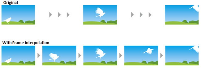
When we watch movies and TV shows online today, most of them are at 24FPS format. As most of our screens like monitors or televisions are in 60FPS or even 120FPS or higher. Figure 1 shows an example of video interpolation. We will see some common artifacts on the screen if we watch these videos on our screen. The reason for the artifacts occurring is because low frame rate video will lose details during the movement.
To avoid these common artifacts, we want to create a program that is powered by Video Frame Interpolation technology to convert 24FPS video to 60FPS one. Video Frame Interpolation is a technology that aims to generate non-existent frames in-between the original frames. The usage of this technology can be used in not only frame rate up-conversion but also the slow-motion video.
Traditional video frame interpolation methods use estimated optical flow to predict the movement of an object between input frames and synthesized intermediate frames. However, the performance varies depending on the quality of the optical flow. Furthermore, the optical flow method is still challenged to generate high-quality frames due to large motion and occlusions.
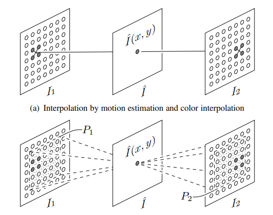
Since this project aims to produce a high-quality frame between existing frames, we decide to use the kernel-based method to predict the frame. This method is to estimate spatially-adaptive convolution kernels for each output pixel and convolve the kernels with the input frames to generate a new frame. Specifically, for each pixel in the interpolated frame, this method takes two receptive field patches centered at that pixel as input and estimates a convolution kernel. The difference between these two methods is shown in Figure 2.
As you can see in Figure 3, the object moves from one frame to the next frame. The model uses the kernel to draw the missing frame and then insert it in-between these two frames. The CNN network generates the missing frame with the other two frames as input.
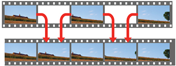
For the test part, we use 60FPS frames videos to train our model, as shown in Figure 4. Each video in the data set is processed in three sets of frames: t, t+1, t+2, where t is from frame 1 to frame 58. We use the frame t and frame t+2 as input and frame t+1 as ground truth. The output frame is used to compare with the original frame t+1 to train the model.
Traditional methods use optical flow for frame interpolation. However, in general, optical flow cannot be calculated from images with ambiguity (known as the aperture problem[7] in computer vision); additional constraints are needed to find a unique solution. Therefore, the quality of the interpolation heavily depends on the accuracy of the flow estimation. It is important to note that this work implements the work of Niklaus et al.[1] in Adaptive Separable Convolution, which claims high-quality results on the video frame interpolation task. We design a convolutional neural network to estimate a proper convolutional kernel to synthesize each output pixel in the interpolated images. Instead of implementing optical flow-based interpolation, our method captures both the motion and interpolation coefficients, generates the kernel through convolution layers, and synthesizes an intermediate video frame.
Our neural network can be trained using widely available video data which provides a sufficiently large training dataset. The main advantages of our method are:
- It achieves better transformation learning and better results;
- Traditional video CODEC requires a lot of manual design on algorithms, while our model provides the ability to automatically learn without being explicitly programmed. However, there is a disadvantage of generating a large kernel for each pixel that it requires an enormous amount of graphics memory.
There are several steps towards making the project. First, We read some related articles and look into previous works on video frame interpolation. We bring traditional video coding algorithms into this project, and adapt them into machine learning algorithms. Then, we can decide which approach we can take to predict inter-frame images.
Second, we need to decide which dataset to be used to train and test the neural network. Since we plan to convert lower FPS videos to 60FPS or 90FPS, we need to find some native 60FPS and 90 FPS video or corresponding picture frames.
Meanwhile, we implement the research method of Niklaus et al. from scratch by using Keras library on Ubuntu 18.04 with Anaconda. Also, we output image demos from the prediction model for quantitative analysis and then generate videos for visual comparison and the in-class presentation.
Finally, we run an experiment on our predicted frames. The metrics including MSE, PSNR, and SSIM, are used to quantify the results and evaluate the performance. A final report is conducted to summarize our experience results.
We develop a deep neural network based on the Adaptive Convolution Network of Niklaus et al. As illustrated in Figure 5 (Niklaus 2017 CVPR), the convolution layers take in two receptive fields, R1 and R2, from two consecutive frames respectively.
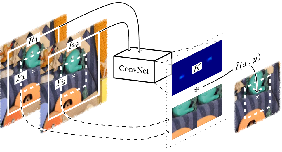
The convolutional model is trained to output a kernel K, which is used with the corresponding patches, P1 and P2, centered in receptive fields, to compute the interpolated frame's output pixel I_hat. The formula for calculating the output pixel is shown as below:
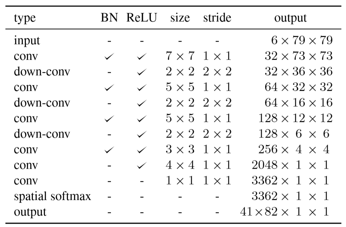
As in Figure 6 (Niklaus 2017 CVPR), we use an identical model like the one Niklaus et al. used in their paper. We also use two receptive blocks with size 79 x 79 x 3 combined to 79 x 79 x 6 as input. In each convolution layer, we use ReLu as our activation function, as well as batch normalization to ensure the variances for both input and output nodes are the same. Each convolution layer is paired with a max-pooling layer using a ReLu activation, a 2 x 2 filter, and a 2 x 2 stride. In order to get the final output with 41 x 82 x 1 x 1 size, we finally use a fully connected layer with spatial softmax activation to get the output kernel with size 41 x 82 x 1 x 1.
We conduct the training and testing on Ubuntu 18.04 with Anaconda. One Quatro RTX 6000 and two RTX 2070 Super are used to train our model. Because all these graphic cards are RTX series, we can enable the RTX 16-bit optimization which makes our training faster. We implement the model based on Keras. The project also works on Powershell in Windows 10.
We use the triplet dataset from the Vimeo90K dataset to train our model. Vimeo90K is a large-scale, high-quality video dataset with 89,800 video clips downloaded from vimeo.com. The triplet dataset is extracted from 15K video clips selected from Vimeo-90K. The triplet dataset has 73,171 triplets for training, in which each triplet is a 3-frame sequence with a fixed resolution of 448 x 256 pixels. We train our network to predict the middle frame of each triplet. We also found Depth-Aware Video Frame Interpolation uses this dataset as well. Regarding the training data, we use 2/3 on training and 1/3 on validation.
Regarding the testing data, we use both the triplet dataset and the HEVC dataset. More specifically, for the HEVC dataset, we use BlowingBubbles and BasketballDrill datasets to evaluate our model and synthesize the final 50FPS video. Each of the datasets has 500 frames, and we use 250 of these 500 frames as the test input.
In our neural network, we initialize our model parameters by using random initialization and AdaMax optimizer to train the proposed network. For AdaMax optimizer parameters, we set beta1 to 0.9, beta2 to 0.999, and the learning rate to 0.001. We use 128 as the Mini-batch size to minimize the loss function. The maximum epochs number is set to 1000.
We also use EarlyStopping to determine the actual number of epochs in each round of training. We monitor validation loss with 1.0 for Min_delta and 10 epochs for the patience. The program saves the best model weights into an HDF5 file when EarlyStopping is triggered.
Regarding the training method, we transform images into blocks and patches to train the model. Also, we use mini-batch to reduce memory costs and improve training efficiency. Three framesets which contain 9 frames in total are used for training at a time. Since we have generated a block and a patch for every pixel on a frame, the block memory and patch memory come to a high cost, which is about 7.3 GB and 2 GB per frame, then a total 22 GB and 6 GB per set.
Training Result
During our training, it takes about 150 seconds to complete one epoch. And the CNN model we finally get contains 15,842,114 parameters in total.
| #Parameters (million) | Runtime per Epoch (seconds) |
|---|---|
| 15.8 | 150 |
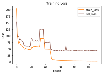
When we train our model with the images of the same scene, the training loss continues to decrease within 20 epochs. After the following climbing halted around epoch #40, the training loss drops again with experience and eventually keeps at a point of stability after epoch #100. The validation loss follows the trend of training loss, but a gap remains between these two curves.
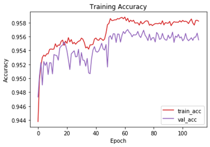
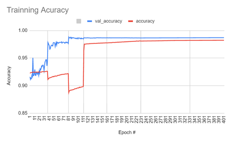
Regarding the accuracy, both training and validation have a similar ascending trend, although there is stagnancy and small drop between epochs #20 and #50 before they eventually climb to a stable higher level.
Figure 7: (a) The training loss and validation loss show the training set maybe is small relative to the validation dataset.
(b) The training accuracy and validation accuracy shows a fair good performance
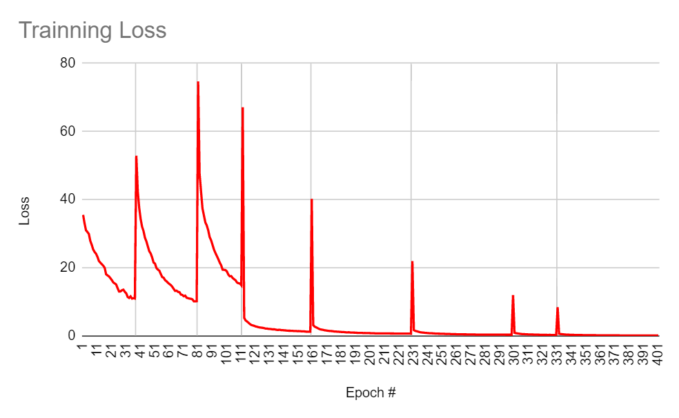
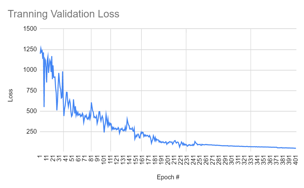
When we train our model with the images of different scenes, the training loss continues to decrease within the epochs in which the images are from the same scenes. But the loss value will jump sharply when the epoch switches to the images from different scenes. Such a phenomenon is called catastrophic forgetting because the change of the training data is so significant that the model has to forget previous experience to fit the new data. However, the validation loss has a pretty much smooth trace without sharp jumping during its descending.
The training accuracy steps down in the first about 100 epochs but quickly rebounds and stays at a much higher level. Though the validation accuracy steadily climbs to the plateau and gets stable after epoch #110.
Figure 8: (a) The training loss has sharp jump while the training data change significantly. It indicates that the training set maybe is small relative to the validation dataset.
(b) The validation loss shows a relative smooth descending trend.
(c) Both of the training accuracy and validation accuracy reach to a good performance while the training accuracy performs poorly at the early stage.
Testing Result
We test our model with Vimeo triplet sets and HEVC data. The table below shows the metrics of MSE, PSNR, and SSIM we got when testing with 100 Vimeo triplet sets which are respectively from the same scene and different scenes.
| 100 Vimeo Triplet Sets | MSE | PSNR | SSIM |
|---|---|---|---|
| Same Scene | 51.3136 | 18.0673 | 0.6097 |
| Different Scenes | 36.9612 | 21.7903 | 0.7966 |
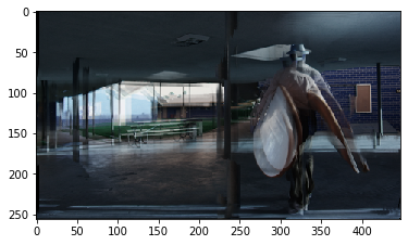
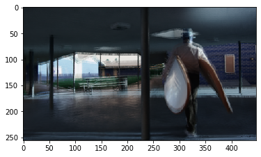
The images below show the interpolated frames generated by our method. The top right image is the interpolated frame based on the frames from the same scene, and the upper left is the ground truth for it. The lower right one is the interpolated frame based on the frames from different scenes, and the lower left is the ground truth for it. As shown in the metric table above and the visual comparison below, the interpolation based on images of the different scene gives a better outcome.
Figure 9 (a) ground truth and the interpolated frame based on images from the same scene
(b) ground truth and the interpolated frame based on images from different scene
As mentioned previously, during the training, the intensive RAM consumption is a huge challenge to our training process, since each consecutive images set (3 frames in total) could take 9GB RAM memory. Therefore, our method only takes in 3 sets of images at a time, and switches to new images sets in the next training section. However, this could lead to an issue called Catastrophic Forgetting, also known as Catastrophic Interference, in Machine Learning. It generally happens when new data is fed to train the model, while the data differs significantly from the previous one. The issue arises because as the CNN model is trained by more data, the model will learn new data quickly and fit them into the model faster than before. In the meantime, the model may forget what it has learnt before.
Unfortunately, we could have avoided this issue at the beginning by simply pre-processing the training data. Instead of feeding 3 sets of images at each time, we could fetch slices of images from different image sets (from different scenes) so that the input data could be diversified.
-
More training data
In this project, we perform 7 rounds of training; for each round, 3 sets of images from different scenes are used. In future research, more data and scenes can be applied to model training. Moreover, we set the patience as 10, which means the training will be terminated if there is no enough improvement in the monitored validation loss within 10 epochs. This model might not be ideal since it goes up or down from one epoch to the next. However, what we care about is that the overall trend is improving, so higher patience value could boost the accuracy of the model, which can be conducted in future training. -
Xavier initialization
Xavier initialization is a method to ensure the variance of both input and output to be the same. The variance of the activation value in training decreases layer by layer, causing the gradient in backpropagation to fall layer by layer. To solve the gradient's disappearance, it is necessary to avoid the reduction of the variance of model weights. An ideal situation is that the output value of each layer maintains a Gaussian distribution. Therefore, the basic idea of Xavier initialization is to keep the variance of the input and output consistent, so as to avoid all output values tending to zero.
Niklaus et al. have proposed a new method in their later research to optimize the memory consumption. As shown in Figure 10 (Niklaus 2017 ICCV), instead of generating a 2-D kernel for each pixel, their new network produces four 1-D kernels for each pixel.
This method is improved by reducing the dimension of the kernel, from one 2-dimension matrix K to two 1-dimension vectors, kh and kv, where they can be used to estimate matrix K. Similar to Formula ?, kh and kv could be rewritten as k1,h, k2,h and k1,v, k2,v respectively. Since we can rewrite the original formula to calculate I(x, y) to Formula ?, the formula to estimate kernel K is Formula ?. In conclusion, each kernel's space complexity will be reduced from O(n^2) to O(2n).
- Ans, B., & Rousset, S. (1997). Avoiding catastrophic forgetting by coupling two reverberating neural networks. Comptes Rendus de l'Académie des Sciences-Series III-Sciences de la Vie, 320(12), 989-997.
- Bao, W., Lai, W. S., Ma, C., Zhang, X., Gao, Z., & Yang, M. H. (2019). Depth-aware video frame interpolation. In Proceedings of the IEEE Conference on Computer Vision and Pattern Recognition (pp. 3703-3712).
- Cote, R. (2016, February 22). Motion Interpolation On TVs: Soap Opera Effect. Retrieved April 26, 2020, from https://www.rtings.com/tv/tests/motion/motion-interpolation-soap-opera-effect.
- Epson Frame Interpolation. (n.d.). Retrieved April 26, 2020, from https://files.support.epson.com/docid/cpd5/cpd52094/source/adjustments/tasks/frame_interpolation.html.
- Florian Raudies (2013) Optic flow. Scholarpedia, 8(7):30724. Retrieved May 10, 2020, from http://www.scholarpedia.org/article/Optic_flow
- Niklaus, S., Mai, L., & Liu, F. (2017). Video frame interpolation via adaptive convolution. In IEEE Conference on Computer Vision and Pattern Recognition (pp. 670-679).
- Niklaus, S., Mai, L., & Liu, F. (2017). Video frame interpolation via adaptive separable convolution. In IEEE International Conference on Computer Vision (pp. 261-270).
- What Is The Soap Opera Effect? - Everything You Need To Know. (2019, June 10). Retrieved April 26, 2020, from https://www.displayninja.com/what-is-the-soap-opera-effect/.

