Overcoming false-positive gene-category enrichment in the analysis of spatially resolved transcriptomic brain atlas data

This is a repository to accompany the manuscript:

Fulcher et al. Nature Communications (2021) 📗 'Overcoming false-positive gene-category enrichment in the analysis of spatially resolved transcriptomic brain atlas data'.

The code below reproduces all statistical tests on gene category enrichment analysis (GCEA) using data from human and mouse.

All data is available for download from the associated Zenodo repository that accompanies this repository. Files that can be downloaded from this repository are labeled in this README using the symbol: 🔗.

Setting up

Data and code for running gene category enrichment analysis (GCEA)

This relies on a Matlab toolbox for GCEA, which can be installed by cloning:

git clone git@github.com:benfulcher/GeneCategoryEnrichmentAnalysis.git

Analyses here require it to be accessible in the path, which can be set by modifying GiveMeFile ('EnrichmentToolbox').

Please follow the instructions from that repository to recompute (or download from the Zenodo repository for this Matlab-GCEA toolbox) the following required data files:

Direct biological process annotations: GOTerms_BP.mat.
Hierarchically propagated annotations (mouse): GOAnnotationDirect-mouse-biological_process-Prop.mat.
Hierarchically propagated annotations (human): GOAnnotationDirect-human-biological_process-Prop.mat.

Data

👤 Human 👤

These files should be placed in the HumanData directory:

Gene-expression data: 100DS360scaledRobustSigmoidNSGDSQC1Lcortex_ROI_NOdistCorrSurface.mat (:link:).
Structural-connectivity data (for case study): HCP_360_20.mat (:link:).

For details on gene-expression data, see this repository.

🐭 Mouse 🐭

These files should be placed in the MouseData directory.

Gene-expression data: AllenGeneDataset_19419.mat (:link:).
Structural connectivity data (for case study): Mouse_Connectivity_Data.mat (:link:).

Data processing and precomputing

Note that batch job scripts for major bulk computations are in the BatchComputing directory. There are files for mouse-related analyses: batchAllMouseAnalyses.sh, and human-related analyses: batchAllHumanAnalyses.sh.

Assembling literature-published enrichment results

Information about enrichment results reported in published studies can be imported and processed by running

ImportLiteratureEnrichment(false,true);

Results are saved as LiteratureEnrichmentLoaded.mat (:link:). Raw data to run this is in the LiteratureEnrichmentData directory (:link:: LiteratureEnrichment.zip).

Generate ensembles of spatially autocorrelated brain maps

Generate random maps that include spatial autocorrelation structure (based on the spatial autocorrelation scale of gene expression as a whole).

plotSummary = true;
GenerateSpatialEnsemble('mouse','all',plotSummary)
GenerateSpatialEnsemble('mouse','cortex',plotSummary)
GenerateSpatialEnsemble('human','cortex',plotSummary)

Saves into the SurrogateMaps/ directory:

human_HCP-cortex_Surrogate_N40000.mat (:link:)
mouse_all_Surrogate_N40000.mat (:link:)
mouse_cortex_Surrogate_N40000.mat (:link:) (for case study)

See also a more comprehensive method for generating spatially autocorrelated brain maps (and matching them to a given phenotype): brainSMASH.

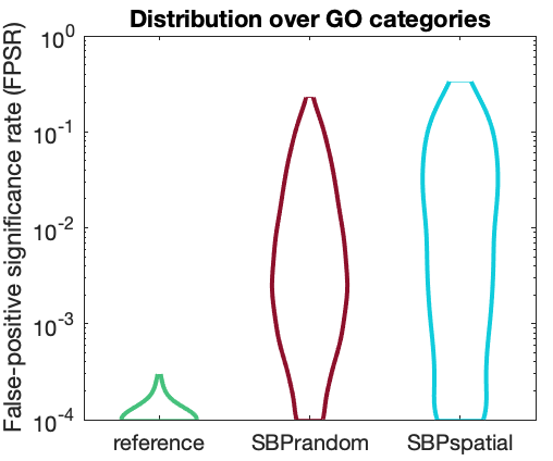
Category False-Positive Rates (CFPRs)

False-positive significance rates can be computed using SurrogateEnrichment (cf. in batchAllHumanAnalyses and batchAllMouseAnalyses).

% Start with default parameters for whole mouse brain:
params = GiveMeDefaultParams('mouse','all');

% Spatially random model (plus independent shuffling of space, separately per gene) [should be no signal---a real null of correlated noise with noise]:
% ('Ref')
params.g.whatSurrogate = 'randomMap';
params.nulls.customShuffle = 'independentSpatialShuffle';
SurrogateEnrichment(params);

% SBP-rand:
params.g.whatSurrogate = 'randomMap';
params.nulls.customShuffle = 'none';
SurrogateEnrichment(params);

% SBP-spatial:
params.g.whatSurrogate = 'spatialLag';
params.nulls.customShuffle = 'none';
SurrogateEnrichment(params);

Then can repeat for human by starting with human cortical parameters (params = GiveMeDefaultParams('human','cortex');)

This saves the following files (to the SurrogateEnrichment directory): (Mouse):

SurrogateGOTables_10000_mouse_randomMap_independentSpatialShuffle.mat 🔗 ('reference').
SurrogateGOTables_10000_mouse_randomMap_none.mat 🔗 ('SBP-random').
SurrogateGOTables_10000_mouse_spatialLag_none.mat 🔗 ('SBP-spatial').

(Human):

SurrogateGOTables_10000_human_randomMap_independentSpatialShuffle.mat 🔗 ('reference').
SurrogateGOTables_10000_human_randomMap_none.mat 🔗 ('SBP-random').
SurrogateGOTables_10000_human_spatialLag_none.mat 🔗 ('SBP-spatial').

The computed results are saved a .mat files and can be read in and processed as a GO Table using SurrogateEnrichmentProcess.

Ensemble-based null distributions

Null distributions for all GO categories is done using the companion Matlab package for both conventional gene-score enrichment and ensemble-based enrichment.

For example, below computes for 'mouse' with the 'randomMap' null model with all other parameters set to defaults:

params = GiveMeDefaultParams('mouse');
params.e.whatEnsemble = 'randomMap';
% Wrapper for running ensemble-based nulls using appropriate gene-expression data:
NullComputation(params);

The null distribution for all GO categories is stored in a table that is saved to a .mat file, in this case: PhenotypeNulls_40000_mouse_randomMap_Spearman_mean.mat. These stored null distributions can then be used for ensemble-based GCEA.

For the analyses presented in the manuscript, these are stored in the EnsembleBasedNulls/ directory:

Human Cortex:

PhenotypeNulls_40000_human-HCP-randomMap_Spearman_mean_.mat ('SBP-random' 🔗)
PhenotypeNulls_40000_human-HCP-customEnsemble_Spearman_mean_.mat ('SBP-spatial' 🔗)

Mouse Brain:

PhenotypeNulls_40000_mouse-all-randomMap_Spearman_mean_.mat ('SBP-random' 🔗)
PhenotypeNulls_40000_mouse-all-customEnsemble_Spearman_mean_.mat ('SBP-spatial' 🔗)

Mouse Cortex (for case study):

PhenotypeNulls_40000_mouse-cortex-randomMap_Spearman_mean_.mat ('SBP-random' 🔗)
PhenotypeNulls_40000_mouse-cortex-customEnsemble_Spearman_mean_.mat ('SBP-spatial' 🔗)

Within-category coexpression

The within-category coexpression metric is precomputed as:

IntraCorrelationByCategory('mouse','geneShuffle',[],'raw',true);
IntraCorrelationByCategory('human','geneShuffle',[],'raw',true);

(although the shuffled versions aren't in any analyses, so the computation on shuffled data is needless).

This saves the results in the DataOutputs/ directory:

Intra_human_geneShuffle_raw_20000.mat (:link:).
Intra_mouse_geneShuffle_raw_20000.mat (:link:).

Compute spatial autocorrelation scores

Compute gene-wise spatial autocorrelation scores for each GO category and each species (cortex/all) (ready for subsequent analysis):

ComputeSpatialEmbeddingScores();

Compute category-wise spatial autocorrelation scores:

SpatialScoringCategories('mouse','all');
SpatialScoringCategories('human','cortex');

This saves to:

CategorySpatialScoring_human.mat (:link:)
CategorySpatialScoring_mouse.mat (:link:)

Analysis

Characterizing Results in the Published Literature

Construct a table of the most commonly reported GO categories:

TopLiteratureCats();

Outputs to SupplementaryTables/LiteratureAnnotations_p005.csv.

For a given GO category of interest, you can find matches to literature using:

LiteratureMatches(whatGOID)

For example, to get information about literature p-values for 'chemical synaptic transmission' (GO:0007268), use LiteratureMatches(7268). Note that for studies that just labeled significant GO categories (and did not provide estimated p-values), these are denoted with a p-value of 0.

Enrichment signatures of ensembles of random spatial phenotypes (and/or including spatial autocorrelation)

Plot distributions of CFPR across GO categories for the three null cases

NullEnrichmentTogether('mouse',true)
NullEnrichmentTogether('human',true)

Saves plots to OutputPlots/CFPR_distributions_mouse.svg and OutputPlots/CFPR_distributions_human.svg.

Generate a table with key statistics of CFPRs in mouse and human

FPSRTable();

Some key statistics are displayed to the command-line, and outputs full annotated table to SupplementaryTables/CFPR_Table.csv.

Investigate the overlap between literature annotations and FPSE as histograms:

As always, the null phenotype ensemble is defined in the GiveMeDefaultParams file.

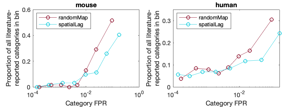
propLitCFPR which looks at how literature-reported categories are distributed across computed levels of CFPR. Outputs figure to OutputPlots/CFPR_Lit_Together.svg.

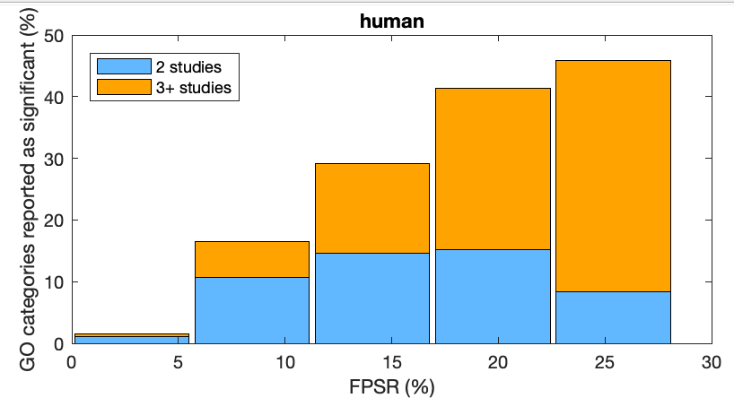
There is also histograms across a linear scale, distinguishing the number of literature analyses flagged across CFPRs:

OverlapLitFPSR('mouse',true)
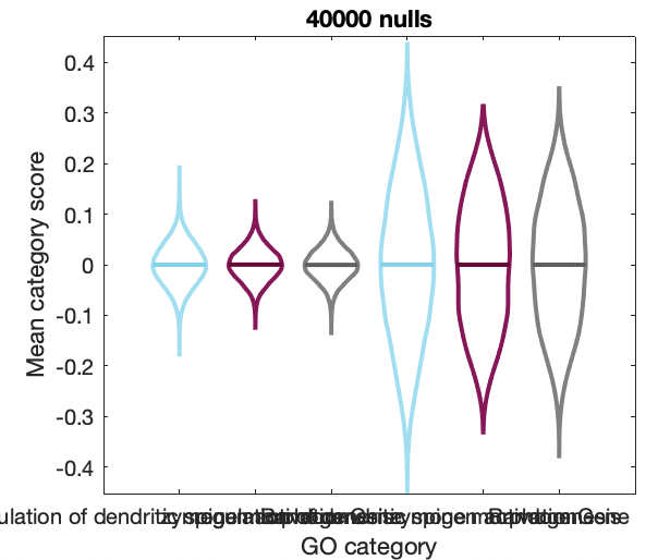
OverlapLitFPSR('human',true)

Specific GO categories

You can zoom into the null score distributions of two specific GO categories (including a random set of 40 genes) using:

PlotCategoryNullCompare('mouse')

The role of within-category coexpression

Generate a table characterizing how within-category coexpression varies across GO categories:

IntraCorrTable();

Outputs to SupplementaryTables/WithinCategoryCoexp.csv.

Does intra-category coexpression relate to CFPR?:

IntraCorrFPSR();

Saves out to OutputPlots/IntraCorr_CFPR.svg.

Do categories with spatially autocorrelated genes exhibit an increase in CFPR against spatially autocorrelated ensembles?

Investigate how CFPR is correlated to gene spatial autocorrelation (by category)

RelativeFPSRAutoCorr()

Saves plot to OutputPlots/Rel_CFPR_SpatialAC.svg.

Save spatial correlation scores to table and get some additional visualizations:

DistanceConfoundResults()

This produces SupplementaryTables/SpatialAutocorrelationScores.csv.

Case Study: Degree

First compute and save all results of conventional GCEA. This will loop through human, mouse-all, and mouse-cortex:

RunConventionalEnrichment();

This saves results files to:

DataOutputs/CaseStudyDegree_human_cortex.mat
DataOutputs/CaseStudyDegree_mouse_all.mat
DataOutputs/CaseStudyDegree_mouse_cortex.mat.

You can then compare the results of all three null models for each setting as:

CaseStudyResults('human','cortex');
CaseStudyResults('mouse','all');
CaseStudyResults('mouse','cortex');

This generates output tables comparing the three types of nulls:

SupplementaryTables/EnrichmentThreeWays_human_cortex.csv
SupplementaryTables/EnrichmentThreeWays_mouse_all.csv
SupplementaryTables/EnrichmentThreeWays_mouse_cortex.csv

There is also CorrelationDegreeCortex to see how genes that differentiate cortical expression are also more likely to be correlated to connectivity degree.

alyssadai/GCEA_FalsePositives