The purpose of this project was to calculate and program joint angles for a six degree of freedom kuka KR210 serial manipulator. The position and orientation of its end effector were provided in a 3-D space. This project uses a Ros environment with Gazebo simulation platform as well as Rviz MoveIt motion planning framework. The intent for the manipulator is to pick up a cylinder from a random location on a shelf and drop it into a bin next to the kuka manipulator.
1. Run the forward_kinematics demo and evaluate the kr210.urdf.xacro file to perform kinematic analysis of Kuka KR210 robot and derive its DH parameters.

Reference frame assignments in URDF file:
| Joint Name | Parent Link | Child Link | x(m) | y(m) | z(m) |
|---|---|---|---|---|---|
| joint_1 | base_link | link_1 | 0 | 0 | 0.33 |
| joint_2 | link_1 | link_2 | 0.35 | 0 | 0.42 |
| joint_3 | link_2 | link_3 | 0 | 0 | 1.25 |
| joint_4 | link_3 | link_4 | 0.96 | 0 | -0.054 |
| joint_5 | link_4 | link_5 | 0.54 | 0 | 0 |
| joint_6 | link_5 | link_6 | 0.193 | 0 | 0 |
| gripper-joint | link_6 | gripper_link | 0.11 | 0 | 0 |
DH Parameters table obtained:
| i | α(i-1) | a(i-1) | d(i) | θ(i) |
|---|---|---|---|---|
| 0 | 0 | 0 | - | - |
| 1 | - 90 | 0.35 | 0.75 | θ1 |
| 2 | 0 | 1.25 | 0 | θ2 |
| 3 | -90 | -0.054 | 0 | θ3 |
| 4 | 90 | 0 | 1.5 | θ4 |
| 5 | -90 | 0 | 0 | θ5 |
| 6 | 0 | 0 | 0.303 | θ6 |
By looking at the kr210.urdf.xacro file we need to determine which relative offset definition between the joints in the urdf file corresponds to their respective DH-parameter. We then extract the DH parameters and anotate them on the table.
2. Using the DH parameter table, you derived earlier, create individual transformation matrices about each joint. In addition, also generate a generalized homogeneous transform between base_link and gripper_link using only end-effector(gripper) pose.
Every joint requires its own transformation matrix which describes the joints position and orientation relative to its prior joint. In order to calculate this matrix, we substitute the DH parameters from the previous table into TF_Matrix function:
def TF_Matrix(alpha, a, d, q):
    TF = Matrix([[cos(q), -sin(q), 0, a],
     [sin(q)*cos(alpha), cos(q)*cos(alpha), -sin(alpha), -sin(alpha)*d],
     [sin(q)* sin(alpha), cos(q)*sin(alpha), cos(alpha), cos(alpha)*d],
     [0,0,0,1]])
    return TF
Sympy's .subs method was used in order to create the appropriate transformation matrices for each joint"
  T0_1 = TF_Matrix(alpha0, a0, d1, q1).subs(DH_Table)
  T1_2 = TF_Matrix(alpha1, a1, d2, q2).subs(DH_Table)
  T2_3 = TF_Matrix(alpha2, a2, d3, q3).subs(DH_Table)
  T3_4 = TF_Matrix(alpha3, a3, d4, q4).subs(DH_Table)
  T4_5 = TF_Matrix(alpha4, a4, d5, q5).subs(DH_Table)
  T5_6 = TF_Matrix(alpha5, a5, d6, q6).subs(DH_Table)
  T6_EE = TF_Matrix(alpha6, a6, d7, q7).subs(DH_Table)
The following are the produced transformation matrices:
Joint 1 T0_1:
[[cos(q1), -sin(q1), 0, 0],
[sin(q1), cos(q1), 0, 0],
[0, 0, 1, 0.75],
[0, 0, 0, 1]]
Joint 2 T1_2:
[[cos(q2 - 0.5*pi), -sin(q2 - 0.5*pi), 0, 0.35],
[0, 0, 1, 0],
[-sin(q2 - 0.5*pi), -cos(q2 - 0.5*pi), 0, 0],
[0, 0, 0, 1]]
Joint 3 T2_3:
[[cos(q3), -sin(q3), 0, 1.25],
[sin(q3), cos(q3), 0, 0],
[0, 0, 1, 0],
[0, 0, 0, 1]]
Joint 4 T3_4:
[[cos(q4), -sin(q4), 0, -0.054],
[0, 0, 1, 1.5],
[-sin(q4), -cos(q4), 0, 0],
[0, 0, 0, 1]]
Joint 5 T4_5
[[cos(q5), -sin(q5), 0, 0],
[0, 0, -1, 0],
[sin(q5), cos(q5), 0, 0],
[0, 0, 0, 1]]
Joint 6 T5_6
[[cos(q6), -sin(q6), 0, 0],
[0, 0, 1, 0],
[-sin(q6), -cos(q6), 0, 0],
[0, 0, 0, 1]]
Joint 7 aka End Effector T6_EE
[[1, 0, 0, a6],
[0, 1, 0, 0],
[0, 0, 1, 0.303],
[0, 0, 0, 1]]
The resulting transformation matrix is as follow:
T0_EE = simplify(T0_1 * T1_2 * T2_3 * T3_4 * T4_5 * T5_6 * T6_EE)After substitution for of 0 for all thetas the resulting matrix for the arm at origin position is as follow:
[[0, 0, 1, 2.153],
[0, -1, 0, 0],
[1, 0, 0, 1.946],
[0, 0, 0, 1]]
3. Decouple Inverse Kinematics problem into Inverse Position Kinematics and inverse Orientation Kinematics; doing so derive the equations to calculate all individual joint angles.
The Kuka KR210’s last three revolute joints of have the same origin and form a spherical "wrist" joint. This allows us to decouple the calculation into two portions, The position kinematics of the wrist center and the orientation kinematics.
r, p , y = symbols('r p y')

ROT_x = Matrix([[1, 0 , 0],
[0, cos(r), -sin(r)],
[0, sin(r), cos(r)]]) # ROLL

ROT_y = Matrix([
[cos(p), 	0 , 	sin(p)],
[0, 		1, 	0],
[-sin(p), 	0, 	cos(p)]]) # PITCH

ROT_z = Matrix([[cos(y), -sin(y), 0],
[sin(y), cos(y), 0],
[0, 0, 1]]) # YAW

ROT_EE = simplify(ROT_z * ROT_y * ROT_x)

Rot_Error = ROT_z.subs(y, radians(180)) * ROT_y.subs(p, radians(-90))

ROT_EE = simplify(ROT_EE * Rot_Error)
Next, we extract end effector rotation and position:
px = req.poses[x].position.x
py = req.poses[x].position.y
pz = req.poses[x].position.z

(roll, pitch, yaw) = tf.transformations.euler_from_quaternion([req.poses[x].orientation.x, req.poses[x].orientation.y, req.poses[x].orientation.z, req.poses[x].orientation.w])
We now calculate the position and orientation of the end effector wrist center
ROT_EE = ROT_EE.subs({'r': roll, 'p': pitch, 'y': yaw})
EE = Matrix([[px], [py], [pz]])
WC = EE - (0.303) * ROT_EE[:,2] We use previously obtained wrist center information to determine theta1
theta1 = atan2(WC[1],WC[0])
side_a = A from figure
side_b = B from figure
side_c = C from figure

side_a = 1.501
side_b = sqrt(pow((sqrt(WC[0] * WC[0] + WC[1] * WC[1]) - 0.35), 2) + pow((WC[2] -0.75),2))
side_c = 1.25

angle_a = acos((side_b * side_b + side_c * side_c - side_a * side_a) / (2 * side_b * side_c))
angle_b = acos((side_a * side_a + side_c * side_c - side_b * side_b) / (2 * side_a * side_c))
angle_c = acos((side_a * side_a + side_b * side_b - side_c * side_c) / (2 * side_a * side_b))

theta2 = pi/2. - angle_a - atan2(WC[2] - 0.75, sqrt(WC[0] + WC[1] * WC[1]) - 0.35)
theta3 = pi/2. - (angle_b + 0.036) # 0.036 accounts for sag in link4 of -0.054mIn order to calculate the remaining thetas, we need to consider an extrinsic rotation sequence. To do so we calculate the rotation matrices as follow:
R0_3 = T0_1[0:3,0:3] * T1_2[0:3,0:3] * T2_3[0:3,0:3]
R0_3 = R0_3.evalf(subs={q1: theta1, q2:theta2, q3: theta3})
The inverse or the rotation matrix is also its transpose as it is an orthogonal matrix.
R3_6 = R0_3.transpose() * ROT_EEWe then calculate the remaining thetas:
theta4 = atan2(R3_6[2,2], -R3_6[0,2])
theta5 = atan2(sqrt(R3_6[0,2]*R3_6[0,2] + R3_6[2,2] * R3_6[2,2]), R3_6[1,2])
theta6 = atan2(-R3_6[1,1], R3_6[1,0])1. Fill in the IK_server.py file with properly commented python code for calculating Inverse Kinematics based on previously performed Kinematic Analysis. Your code must guide the robot to successfully complete 8/10 pick and place cycles. Briefly discuss the code you implemented and your results.
To compute and print matrices we used IK_debug.py. This program was a useful as it quickly allowed the testing of the calculating values.
Once we ran the simulation and moved our results to the IK_server.py it was noticed that the VM lags at certain steps. The longest time was spent during the IK calculations. Although this takes some time in my current computer configurations, it is still successful at picking up the cylindrical pieces from any location on the shell and dropping it its destined location.
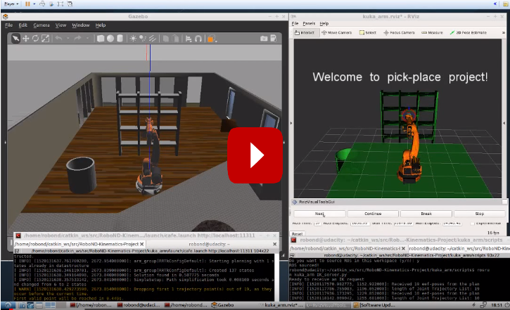
 A video to this project can be found below: