This repo contains all the assignments from the course called EVA conducted by the 'The School Of AI'. Object detection, Object reconisation, segmentation, monocular depth estimation.

- Basics of Python
- Setting Up Basic Skeleton
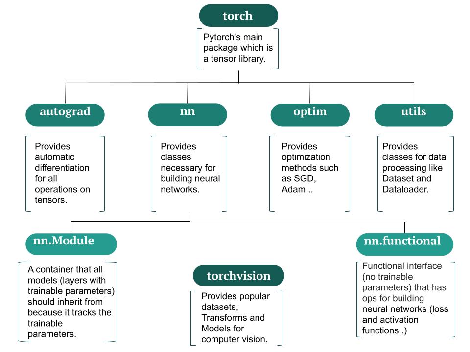
- Pytorch Basics
- To achive 99.4% validation accuracy for MNIST DatSet
- The whole process- Coding drill
- Regularisation techinques on MNIST
- Advanced convolutions(depthwise seperable and dialated convolutions) on CIFAR 10 with advanced image augmentation like utout, coarseDropout
- Vision Transformer
- Training on TinyImageNet
- Object detection in YOLO
- Custom Object detection training in Yolo

EVA Transformerbased Deep Learning course. This repo contains all my nlp work and learning. Made public so that others can learn and get benefits.The repo will contain all my project related to NLP learning and vision model deployment using mediapipe.
The Convolution operation reduces the spatial dimensions as we go deeper down the network and creates an abstract representation of the input image. This feature of CNN’s is very useful for tasks like image classification where you just have to predict whether a particular object is present in the input image or not.
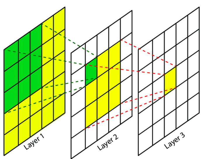
- dilated convolutions are used to increase the receptive field of the higher layers, compensating for the reduction in receptive field induced by removing subsampling.


A scenario of dilated convolution for kernel size 3×3. From the top: (a) it is the situation of the standard convolutional layer when the dilation rate is (1,1). (b) when the dilation rate become (2,2) the receptive field increases. (c) in the last case, the dilation rate is (3,3) and the receptive field enlarges even more than situation b.

The convolution feature might cause problems for tasks like Object Localization, Segmentation where the spatial dimensions of the object in the original image are necessary to predict the output bounding box or segment the object. To fix this problem various techniques are used such as fully convolutional neural networks where we preserve the input dimensions using ‘same’ padding. Though this technique solves the problem to a great extent, it also increases the computation cost as now the convolution operation has to be applied to original input dimensions throughout the network.

In the first step, the input image is padded with zeros, while in the second step the kernel is placed on the padded input and slid across generating the output pixels as dot products of the kernel and the overlapped input region. The kernel is slid across the padded input by taking jumps of size defined by the stride. The convolutional layer usually does a down-sampling i.e. the spatial dimensions of the output are less than that of the input. The animations below explain the working of convolutional layers for different values of stride and padding.

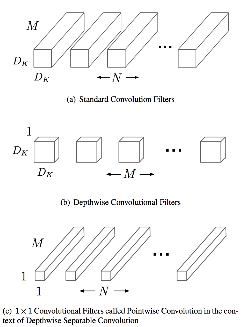
Depthwise Separable Convolutions A lot about such convolutions published in the (Xception paper) or (MobileNet paper). Consist of:
Depthwise convolution, i.e. a spatial convolution performed independently over each channel of an input. Pointwise convolution, i.e. a 1x1 convolution, projecting the channels output by the depthwise convolution onto a new channel space. Difference between Inception module and separable convolutions:
Separable convolutions perform first channel-wise spatial convolution and then perform 1x1 convolution, whereas Inception performs the 1x1 convolution first.
depthwise separable convolutions are usually implemented without non-linearities.
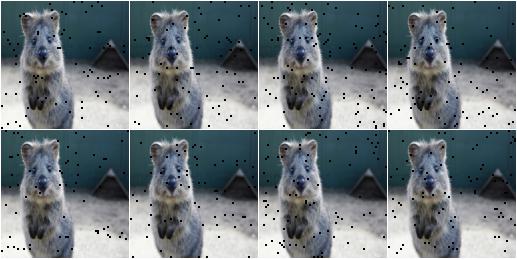
Coarse Dropout and Cutout augmentation are techniques to prevent overfitting and encourage generalization. They randomly remove rectangles from training images. By removing portions of the images, we challenge our models to pay attention to the entire image because it never knows what part of the image will be present. (This is similar and different to dropout layer within a CNN).
- Cutout is the technique of removing 1 large rectangle of random size
- Coarse dropout is the technique of removing many small rectanges of similar size.
Example. Drop 2% of all pixels by converting them to black pixels, but do that on a lower-resolution version of the image that has 50% of the original size, leading to 2x2 squares being dropped:
import imgaug.augmenters as iaa
aug = iaa.CoarseDropout(0.02, size_percent=0.5)
Cyclic learning rates (and cyclic momentum, which usually goes hand-in-hand) is a learning rate scheduling technique for (1) faster training of a network and (2) a finer understanding of the optimal learning rate. Cyclic learning rates have an effect on the model training process known somewhat fancifully as "superconvergence".
To apply cyclic learning rate and cyclic momentum to a run, begin by specifying a minimum and maximum learning rate and a minimum and maximum momentum. Over the course of a training run, the learning rate will be inversely scaled from its minimum to its maximum value and then back again, while the inverse will occur with the momentum. At the very end of training the learning rate will be reduced even further, an order of magnitude or two below the minimum learning rate, in order to squeeze out the last bit of convergence. The maximum should be the value picked with a learning rate finder procedure, and the minimum value can be ten times lower.
Cyclic learning rates (and cyclic momentum, which usually goes hand-in-hand) is a learning rate scheduling technique for (1) faster training of a network and (2) a finer understanding of the optimal learning rate. Cyclic learning rates have an effect on the model training process known somewhat fancifully as "superconvergence".
To apply cyclic learning rate and cyclic momentum to a run, begin by specifying a minimum and maximum learning rate and a minimum and maximum momentum. Over the course of a training run, the learning rate will be inversely scaled from its minimum to its maximum value and then back again, while the inverse will occur with the momentum. At the very end of training the learning rate will be reduced even further, an order of magnitude or two below the minimum learning rate, in order to squeeze out the last bit of convergence. The paper suggests the highest batch size value that can be fit into memory to be used as batch size. The author suggests , its reasonable to make combined run with CLR and Cyclic momentum with different values of weight decay to determine learning rate, momentum range and weigh decay simultaneously. The paper suggests to use values like 1e-3, 1e-4, 1e-5 and 0 to start with, if there is no notion of what is correct weight decay value. On the other hand, if we know , say 1e-4 is correct value, paper suggests to try 3 values bisecting the exponent( 3e-4, 1e-4 and 3e-5).

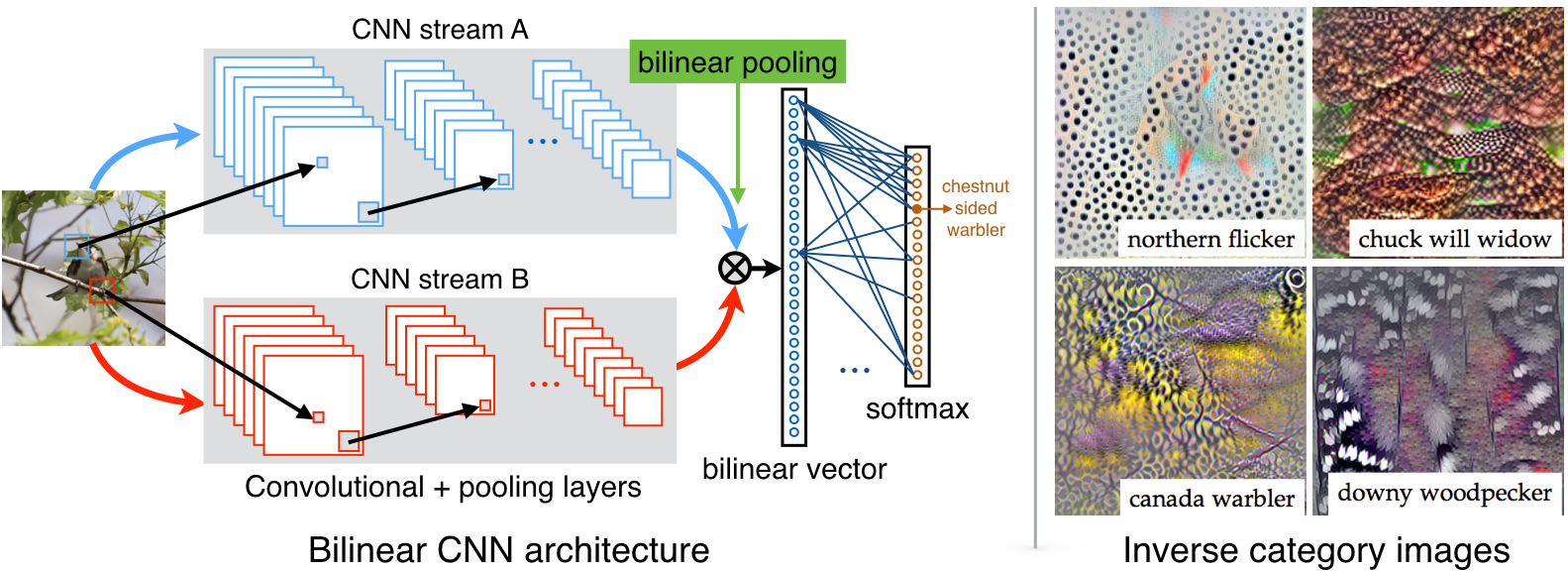
Fine-grain visual classification (FGVC) refers to the task of distinguishing the categories of the same class. ... Fine-grained visual classification of species or objects of any category is a herculean task for human beings and usually requires extensive domain knowledge to identify the species or objects correctly. Refer the video https://www.youtube.com/watch?v=s437TvBuziM
Fine-Grained Image Classification (FGIC) with B-CNNs


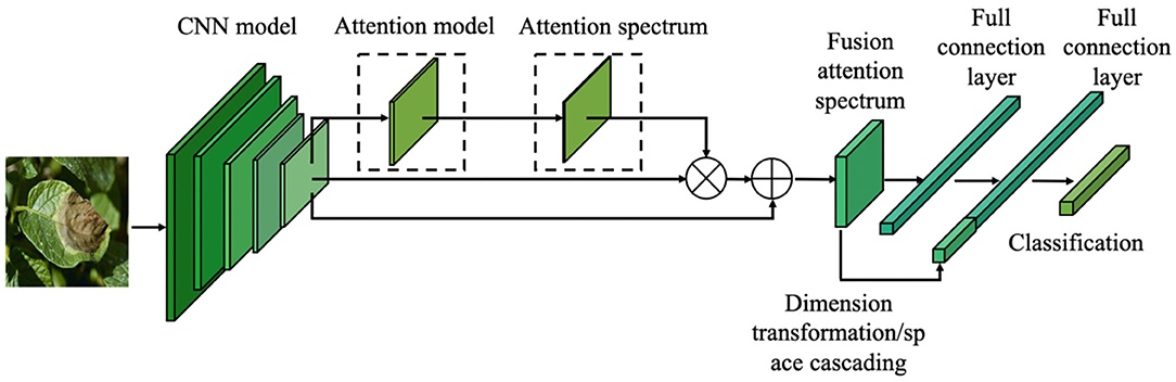
Fine-Grained Image Classification for Crop Disease Based on Attention Mechanism
he Receptive Field (RF) is defined as the size of the region in the input that produces the feature[3]. Basically, it is a measure of association of an output feature (of any layer) to the input region (patch). The idea of receptive fields applies to local operations (i.e. convolution, pooling).A convolutional unit only depends on a local region (patch) of the input. That’s why we never refer to the RF on fully connected layers since each unit has access to all the input region. To this end, our aim is to provide you an insight into this concept, in order to understand and analyze how deep convolutional networks work with local operations work. In essence, there are a plethora of ways and tricks to increase the RF, that can be summarized as follows:
- Add more convolutional layers (make the network deeper)
- Add pooling layers or higher stride convolutions (sub-sampling)
- Use dilated convolutions
- Depth-wise convolutions Refer the article https://theaisummer.com/receptive-field/
Understanding the receptive field of deep convolutional networks