gnlse

Rev 19, 28.12.2014

a python script to simulate the propagation of pulses in optical fibers
the generalized Nonlinear Schroedinger Equation (gNLSE) is modeled

integration is done via SCIPYs ode solvers (adaptive stepsize)
it is derived from the RK4IP matlab script written by J.C.Travers, H. Frosz and J.M. Dudley that is provided in "Supercontinuum Generation in Optical Fibers", edited by J. M. Dudley and J. R. Taylor (Cambridge 2010).
see http://scgbook.info/ for the original script.

available demos (demos.py):

Raman shift (soliton self frequency shift)
self-steepening
higher-order soliton
soliton self-frequency shift cancellation
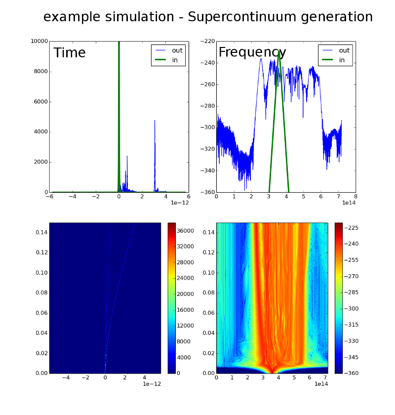
supercontinuum generation via soliton fission
compare the different Raman response models available (not actually a simulation but a temporal and spectral plot)
losses (simple, independent of frequency)
frequency dependent losses (N=1 soliton center frequency changes)

required python packages:

you will need recent (!) versions of

numpy
scipy
matplotlib (which is not necessarily needed for simulations, but required for function 'inoutplot')
optictools (like above, only required by 'inoutplot'); it can be found on (github/xmhk)

have a look at http://www.scipy.org/ and grab the lastest stable versions

basic usage:

please have a look at demos.py

use prepare_sim_params() to prepare a time and frequency grid; declare things like the fiber's dispersion, losses, the nonlinear effects that have to be considered, etc
calculate your input field (in the time domain)
use perform_simulation to propagate your field
saveoutput can save the simulated data in a matlab-style file
loadoutput does the reverse thing
inoutplot can give you a quick overview (temporal and spectral in/output, false-color plot of temporal and spectral evolution)

function reference (still incomplete)

Functions you need to access from outside

prepare_sim_params(alpha, betas, centerwavelength, gamma, length, N, [OPTIONAL ARGUMENTS])

arguments (give in this order):
- alpha - loss coefficient (1/m) or vector
- betas - list or vector [beta0, beta1, beta2]
- center wavlength (m)
- gamma (1/(W*m))
- fiber length (m)
- N - number of time/frequency discretization poins (factors of 2 recommended)
- tempspread (numerical factor, how to spread the time window, 1.0 recommended)
optional arguments
- zpoints : number of output z-steps
- raman True/False : include the raman effect? Standard is False
- ramantype: choose different raman response functions:
  - 'blowwood' Blow and D. Wood, IEEE J. of Quant. Elec., vol. 25, no. 12, pp. 2665–2673, Dec. 1989.
  - 'linagrawal' Lin and Agrawal, Opt. Lett., vol. 31, no. 21, pp. 3086–3088, Nov. 2006.
  - 'hollenbeck' (Standard) Hollenbeck and Cantrell J. Opt. Soc. Am. B / Vol. 19, No. 12 / December 2002
- fr - fraction of non-instantaneous raman response. From the literature we find:
  - blowwood usually fr = 0.18
  - linagrawal fr = 0.245
  - hollenbeck models the experimental data quite accureate. fr should be around 0.2
- shock term True/False - include shock term? Default False
- nsteps - maximum number of steps for one ode-integration (standard 500)
- statusmsg: whether to show status True/False
- status_update_intv : when statusmsg == True, print status only every nth step (n=status_update_intv)
- reltol - ode-solver relative accuracy parameter (standard 1e-6)
- abstol - ode-solver absolute accuracy parameter (standard 1e-9)
- integratortype: choose one of
  - 'dop853'
  - 'dopri5'
  - 'lsoda'
  - 'vode' see corresponding section in the scipy docs. Standard is dopri5
output:
- a simparams dict

perform_simulation( simparameters, inifield )

integrates the gNLSE

arguments:
- simparameters: a simparam dict created by prepare_simparams
- inifield: the electrical field in the time domain
ouput:
- a timefield array(size: N times zpoints+1)
- a freqfield array(size: N times zpoints+1)
- a z-vector

saveoutput(filename):

saves the output (temporal and spectral field, some simparams in one matlab-style file

    INPUT:
    - filename
    - timefieldarray
    - freqfieldarray
    - zvec
    - simparams dict
    
    the saved dict will contain the following fields:
    - tvec time vector
    - omvec omega vector (absolute)
    - relomvec omega vector (relative)
    - om0 center frequency
    - betacurve dispersion vector
    - length fiber length
    - zpoints number of z steps
    - points time vector points
    - timefield array of field (temporal domain)
    - freqfielf array of field (spectral domain)
    - zvec z vector
    - tfield1, tfield2 in- and output field (temporal domain)
    - ffield1, ffield2 in- and output field (spectral domain domain)

loadoutput(filename)

load output saved by 'saveoutput'

    INPUT:
    - filename
    
    OUTPUT:
    - a dictionary containing the fields:
        - tvec time vector
        - omvec omega vector (absolute)
        - relomvec omega vector (relative)
        - om0 center frequency
        - betacurve dispersion vector
        - length fiber length
        - zpoints number of z steps
        - points time vector points
        - timefield array of field (temporal domain)
        - freqfielf array of field (spectral domain)
        - zvec z vector
        - tfield1, tfield2 in- and output field (temporal domain)
        - ffield1, ffield2 in- and output field (spectral domain domain)

extract_outfield_from_dict( outpdict )

extract only the output field (time, freq)
and the freq vectors from a dict created
by mydict  = loadoutput(filename)

returns a Nx7 numpy.array

output_field( M )

a quick way to get an output field 
from a numpy.array extract_outfield_from_dict

returns an OBJECT with the variables

- self.tvec
- self.omvec
- self.relomvec
- self.nuvecthz
- self.tfield
- self.ffield
- self.Som   energy density (with respect to rad/s)
- self.Snu   energy density (with respect to Hz)

inoutplot

plot the input and output (both domains) as well as temporal and spectral evolution into one figure

    INPUT:
    - d: dictionary created by 'loadoutput'
    
    OPTIONAL INPUT:
    - zparams: dict that may contain the fields
       - 'fignr':fignr
       - 'clim':(cl1,cl2)    limit for colorcode (z) limits
       - 'fylim':(fyl1,fyl2) y-limit for spectral plot
OUTPUT:
- ax1,ax2,ax3,ax4 handles of the four subfigures

Internal functions (you usually don't have to call by yourself)

TDB - to be documented ;)

anates/gnlse