The Self-Organising Map (SOM) is a type of Artificial Neural Network (ANN) first proposed by Finnish scientist Teuvo Kohonen in 1982. It’s main uses are in data clustering and dimensionality reduction. Features with any number of attributes are projected onto a lower-dimensional neural network (commonly 1-, 2- or 3-dimensional) for the purpose of simplification, visualisation or pattern analysis. In order to improve it’s usefulness for spatial data science, the SOM can be modified to consider geographic proximity during it’s learning. The result is clustering that is geographically coherent and can provide additional insights into the source data.
The spatially aware SOM (GeoSOM) was developed at the New University of Lisbon (UNL) in the early 2000s and a software suite was created in MATLAB. The software installer requires Windows and the source code consists of MATLAB .m files. Thus, a free and open-source implementation is currently not available to researchers or the public.
Example data has been created for the GeoSOM Suite to demonstrate the capabilities of the MATLAB-based GeoSOM software developed at UNL. Available at GeoSOM Repository (Lobo, 2009), two of the datasets are included here. Both datasets have a single non-spatial attribute, such that clustering would depend entirely on this property in the traditional SOM. Using the GeoSOM, however, we expect the clustering to also be partially spatially dictated. The third dataset consists of real-world demographic metrics and tests the true functionality of the GeoSOM.
*Squareville is an artificial dataset purposely created to use in GeoSOM suite. Squareville is a small-town with square boundaries and an area of 10000 m2. Squareville has 100 houses evenly spaced with coordinates x in [5, 95] and y in [5, 95]. For each house we know the average salary, which is s in [900 1000] for 35<=x<=65 and s in [0 100] * This simple scenario consists of 100 houses in a regular grid. Roughly divided into thirds, the first and last third have significantly lower values for “average salary” than the middle third. Traditional clustering simply yields two clusters, for rich and poor (high and low values). Incorporating a geographic constraint, we expect the poor cluster to differentiate into an “eastern” and a “western” poor area.
*The points follow a uniform distribution in the geographical coordinate, within the rectangle limited by [(0,0),(20,5)]. In the non-geographical dimension there are three zones of high spatial autocorrelation, where the values of z are very similar among neighbouring points, with a uniform in [90,91] in two zones and [10,11] in another. There is also one area of “negative autocorrelation”, where half the data points have z==0 and the other half have z==90. In the rest of the input space z has a uniform distribution in [0,100]. * This feature space has 5000 points in a regular grid, with five distinct zones (also based on a single non-spatial attribute). Simple SOM clustering would group these points according to value only, whereas we would expect the GeoSOM to create geographically separate clusters in the four corners as well as (depending on the model parameterisation) within the one corner with high negative autocorrelation.
The 2011 Portugal Census data contains the centroid coordinates and 11 selected socio-economic variables for the 278 municipalities of Portugal. A conventional SOM would classify municipalities solely on socio-economic metrics. For example, highly urbanised municipalities would be grouped together regardless of geographic proximity, because of similar socio-economic characteristics. The same is true for various levels of rural municipalities. We expect the GeoSOM classification to differentiate between Lisbon, Porto and Coimbra. We also expect the final result to produce contiguous clusters of data points.
The GeoSOM takes an additional parameter k, which can be defined as the spatial weight. With k=0 space is disregarded and the GeoSOM functions exactly as a traditional SOM. As the value of k increases, spatial proximity increases in significance. With k=1, the feature space and geographic space have equal weight. To incorporate this constraint Bacao et al (2004) filtered neurons by proximity during every learning iteration and the best matching unit (BMU) could only be selected from a proximal subset of all the neurons in the map. Thus, with a single feature selected, the geographic distance to every neuron is calculated and distal neurons are excluded from consideration. Then the vector distances in the feature space are calculated (as per the normal routine) and the BMU selected. The rest of the learning process is identical to a conventional SOM.
In this package, the geographic space is regarded as a separate data layer with modifiable importance (k). The function geosom is a wrapper for the supersom routine (similar to som and xyf in the kohonen package). The user passes the data along with the weight k, and the labels of any coordinate columns in the data frame. The user also specifies whether non-spatial data should be normalised. The geosom function strips the spatial data into a separate data frame and does not normalise it. Non-spatial data is normalised if requested, and supersom is called with normalizeDataLayers set to FALSE.
For demonstration and consistency, a hexagonal grid of 5x4 neurons is used in the first two examples. In the Portugal dataset, a 6x10 hexagonal grid is used.
library(kohonen)
library(Rcpp)# geosom function
# call geosom by specifying data, coordinate labels, and spatial weight
# data as data.frame
# coords as a list of coordinate column labels
# k as a decimal number from 0 to 1
# norm as Boolean
"geosom" <- function(data, coords, k, norm, ...) {
# subset spatial data
geodata = data.matrix(data[,(names(data) %in% coords)])
# subset non-spatial data
data = data.matrix(data[,!(names(data) %in% coords)])
spatial.weight = c(1, k)
# if data to be normalised, we do it here
# xyz cannot be scaled disproportionately
if (isTRUE(norm)) {
data = scale(data)
}
# disregard geography if spatial weight is zero
if (k==0) {
supersom(list(data), normalizeDataLayers=FALSE, ...)
} else {
supersom(list(data, geodata), user.weights=spatial.weight, normalizeDataLayers=FALSE, ...)
}
}
"geosomgrid" <- function(x,y) {
somgrid(x,y,"hexagonal", "gaussian")
}# Parameterisation
som_x = 5 # neural map horizontal size
som_y = 4 # neural map vertical size
norm = TRUE # normalise input data
set.seed(151) # to ensure reproducibility,
# but is apparently ineffective here
minor.grid = geosomgrid(som_x, som_y) # neural map grid
major.grid = geosomgrid(2*som_x, 2*som_y) # neural map gridThis is a utility function to view SOM results at a glance, with 6 plot types displayed in a single figure.
# plot function 3 x 2
"show_results" = function(kohobj) {
  par(mfrow = c(2, 3))
  codes = getCodes(kohobj)
  # in the case of >1 attribute, only the first is plotted in "property" plot
  if (is.list(codes)) {
    plot(kohobj, type = "codes", whatmap = 1, shape="straight")
    plot(kohobj, type = "property", property = codes[[1]][, 1], shape="straight")
  } else {
    plot(kohobj, type = "codes", shape="straight")
    plot(kohobj, type = "property", property = codes[, 1], shape="straight")
  }
  plot_types = c("mapping", "counts", "dist.neighbours", "changes")
  for (plot_type in plot_types) {
    plot(kohobj, type = plot_type, shape="straight")
  }
}# Data
data(squareville)
head(squareville)## X Y S
## 1 5 5 951
## 2 5 15 993
## 3 5 25 923
## 4 5 35 926
## 5 5 45 929
## 6 5 55 998
# Conventional SOM:
som.model = som(data.matrix(squareville$S), grid = minor.grid)
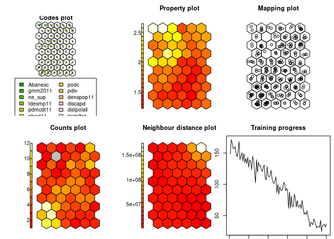
show_results(som.model)
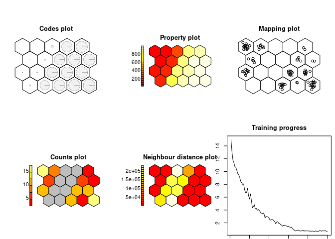
The conventional SOM produces a very clear binary classification, based on the single non-spatial variable S, into a low- and a high-value cluster.
# GeoSOM:
geosom.model = geosom(data = squareville,
                      coords = c("X", "Y"),
                      k=3,
                      norm = norm,
                      grid = minor.grid)
show_results(geosom.model)
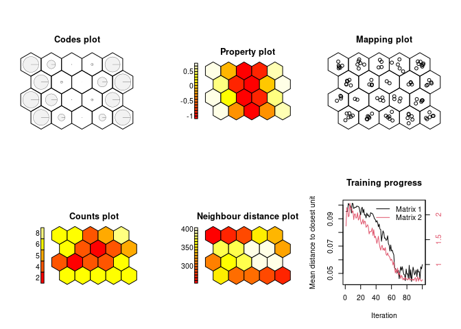
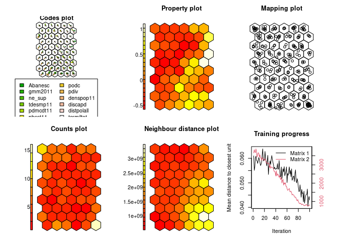
The GeoSOM produces three distinct clusters: one low-value, and two spatially separated high-value clusters.
# Data:
data(four_corners)
head(four_corners)
## X Y L
## 1 2.59 11.85 10.88
## 2 17.15 10.96 90.06
## 3 3.01 10.31 10.33
## 4 8.65 5.87 52.33
## 5 14.35 7.77 49.93
## 6 10.71 7.74 94.99
# Conventional SOM:
som.model = som(data.matrix(four_corners$L), grid = minor.grid)
show_results(som.model)
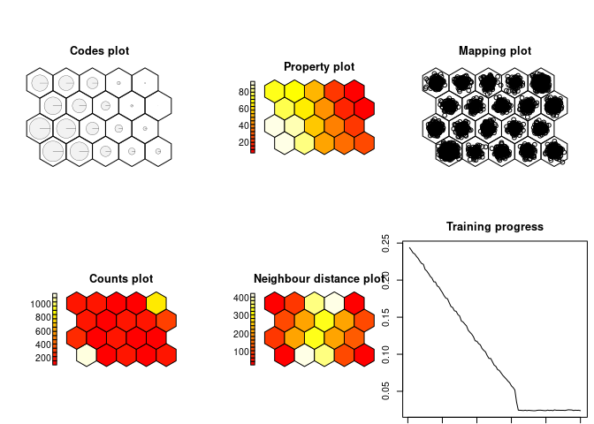
Similar to the Squareville result, the conventional SOM produces a binary classification into a low- and a high-value cluster. However, the distinction is more gradual and a third cluster of intermediate values may also be discerned.
# GeoSOM:
geosom.model = geosom(data = four_corners,
                      coords = c("X", "Y"),
                      k = 3,
                      norm = norm,
                      grid = minor.grid)
show_results(geosom.model)
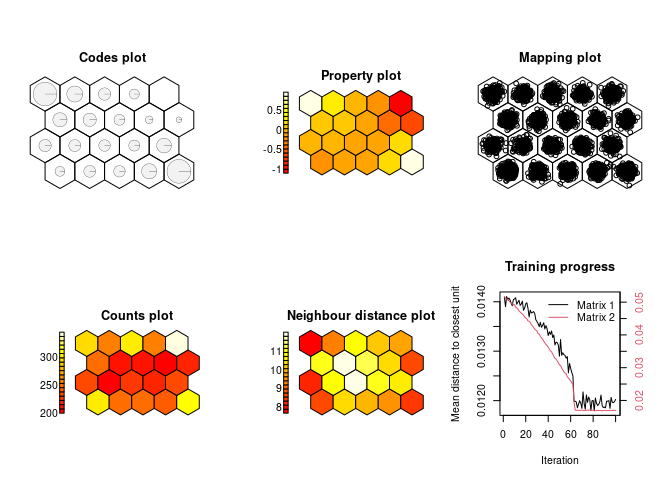
The GeoSOM results are more open to interpretation but show four very distinct clusters. A fifth and sixth may also be defined, each with increasingly fuzzy boundaries.
# Data:
data(project3)
head(project3)
## Abanesc gmm2011 ne_sup tdesmp11 pdmcdt11 pbsst11 podc pdiv denspop11
## 1 1.97 969.71 10.253651 13.6 0.059888 0.742530 86.8 0.203433 55.02378
## 2 1.48 919.96 9.725704 10.1 0.034679 0.328940 85.2 0.272371 142.35820
## 3 0.97 692.25 4.648293 8.9 0.229984 0.749132 61.6 0.073086 26.46953
## 4 0.70 764.72 4.982619 15.6 0.069160 1.112442 57.1 0.102687 10.76697
## 5 1.25 909.51 9.518236 10.4 0.225804 0.300966 80.2 0.205924 158.99260
## 6 1.96 913.89 11.494990 17.2 0.118196 0.991966 102.8 0.259626 290.25194
## discapd distpolall tcrmiltot centroidx centroidy
## 1 49813.7 6763.774 26.39542 -2125.85 -26872.2
## 2 23220.1 6135.107 32.16074 -22224.80 101936.0
## 3 32855.2 6166.988 23.20482 51046.80 123750.0
## 4 46776.2 6664.486 16.94335 65335.10 -116583.0
## 5 15457.6 4488.527 34.01711 -30628.40 114637.0
## 6 30102.4 3083.984 103.62986 -8846.02 -281339.0
# initialise a special grid for larger dataset
# 'landscape' orientation to accommodate Portugal's geography
pt_grid = geosomgrid(6,10)
# Conventional SOM:
som.model = som(data.matrix(project3[,!(names(project3) %in% c("centroidx","centroidy"))]),
                grid = pt_grid)
show_results(som.model)
The SOM yields 5-7 classes (depending on interpretation). Classes have comparatively fuzzy borders, which is expected of real demographic data. Lisbon’s and a few of Porto’s municipalities are the most distant from other classes, with many socio-economic metrics that are orders of magnitude removed from the rest of the nation.
# GeoSOM:
geosom.model = geosom(data = project3,
                      coords = c("centroidx","centroidy"),
                      k = 5,
                      norm = norm,
                      grid = pt_grid)
show_results(geosom.model)
In the GeoSOM classification, many more classes can be discerned. Urban regions are geographically classified, as expected. Rural areas that are very close in the feature space are now separated by geographic space. The 60 neurons now yield between 16 and 21 clusters.
In the simple Squareville example, the effect of spatial weight is
obvious. The cluster of high-value data points is split into ‘eastern’
and ‘western’ clusters, allowing more informed conclusions to be drawn.
The 4 Corners example is similar: the single-dimensional non-spatial
data clusters into 3 groups. However, in space it becomes clear that
distinct regional clusters exist, that data analysts should be aware of.
The final example is the most promising, as it pertains to real data and
can be compared to the results of an unpublished project
(man/Project_3.pdf) using GeoSOM Suite (Henriques et al, 2009).
Whilst conventional clustering is very useful for socio-economic data,
the spatially aware SOM results can facilitate many more insights and
increase the significance of the data.
Although the method of spatial constraint is not identical to Bação et al (2004) the results are comparable. A thorough open-source reimplementation of their method requires expertise in C++ and is a part of the future scope of research. However, as demonstrated, this package can deliver excellent results. As with conventional SOMs, there is significant potential for parameterisation and experimentally-inspired calibration.
Bação, F., Lobo, V. and Painho, M., 2004, October. Geo-self-organizing map (Geo-SOM) for building and exploring homogeneous regions. In International Conference on Geographic Information Science (pp. 22-37). Springer, Berlin, Heidelberg.
Henriques, R., Bação, F. and Lobo, V., 2009, June. GeoSOM Suite: A tool for spatial clustering. In International conference on computational science and its applications (pp. 453-466). Springer, Berlin, Heidelberg.
Lobo, V., 2009, March. GeoSOM Repository, viewed 4 September 2022, https://www.isegi.unl.pt/labnt/geosom/georepository/.
Wehrens R, Kruisselbrink J (2018). “Flexible Self-Organizing Maps in kohonen 3.0.” Journal of Statistical Software, 87(7), 1-18. doi: 10.18637/jss.v087.i07 (URL: https://doi.org/10.18637/jss.v087.i07).
Wehrens R, Buydens LMC (2007). “Self- and Super-Organizing Maps in R: The kohonen Package.” Journal of Statistical Software, 21(5), 1-19. doi: 10.18637/jss.v021.i05 (URL: https://doi.org/10.18637/jss.v021.i05).
