CPO data collection, aggregation, and analysis code repository
The primary function of this repository is to provide reproducible scripts for collecting and summarizing water rights and climate data for the state of Colorado.
- CDSS/DWR via cdssr
-
SWE from NRCS SNOTEL sites
-
NRCS streamflow forecasts
-
EDDI (Evaporative Drought Demand Index)
The main script in this repository is the get_everything() script that
when run, will pull together all available data from the sources above
and summarize the data into an annual value for every point (water
right) in each district.
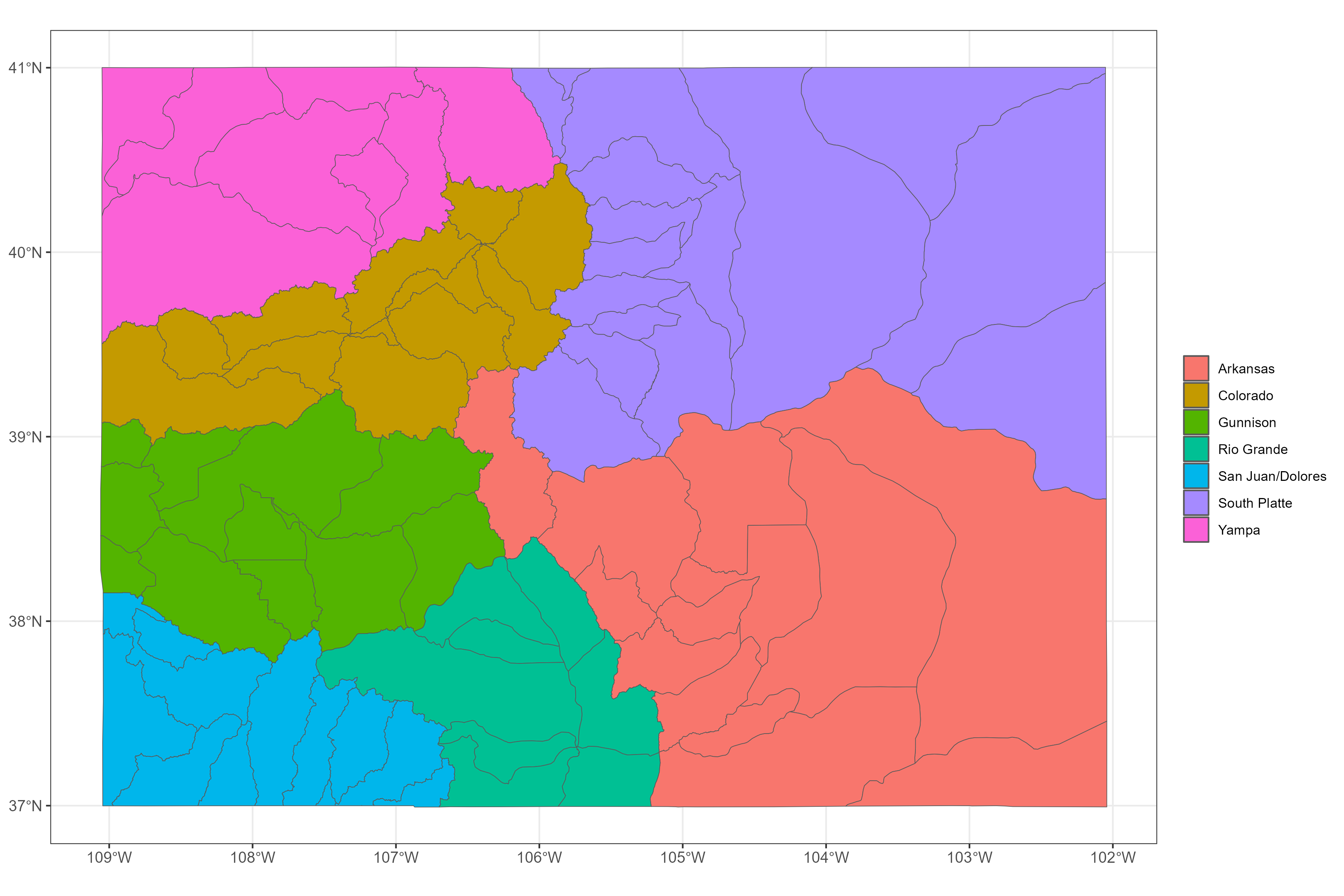
For each water district in Colorado, we collect the same set of water right and climate data indicators. Below is a plot showing the different water district boundaries in Colorado.
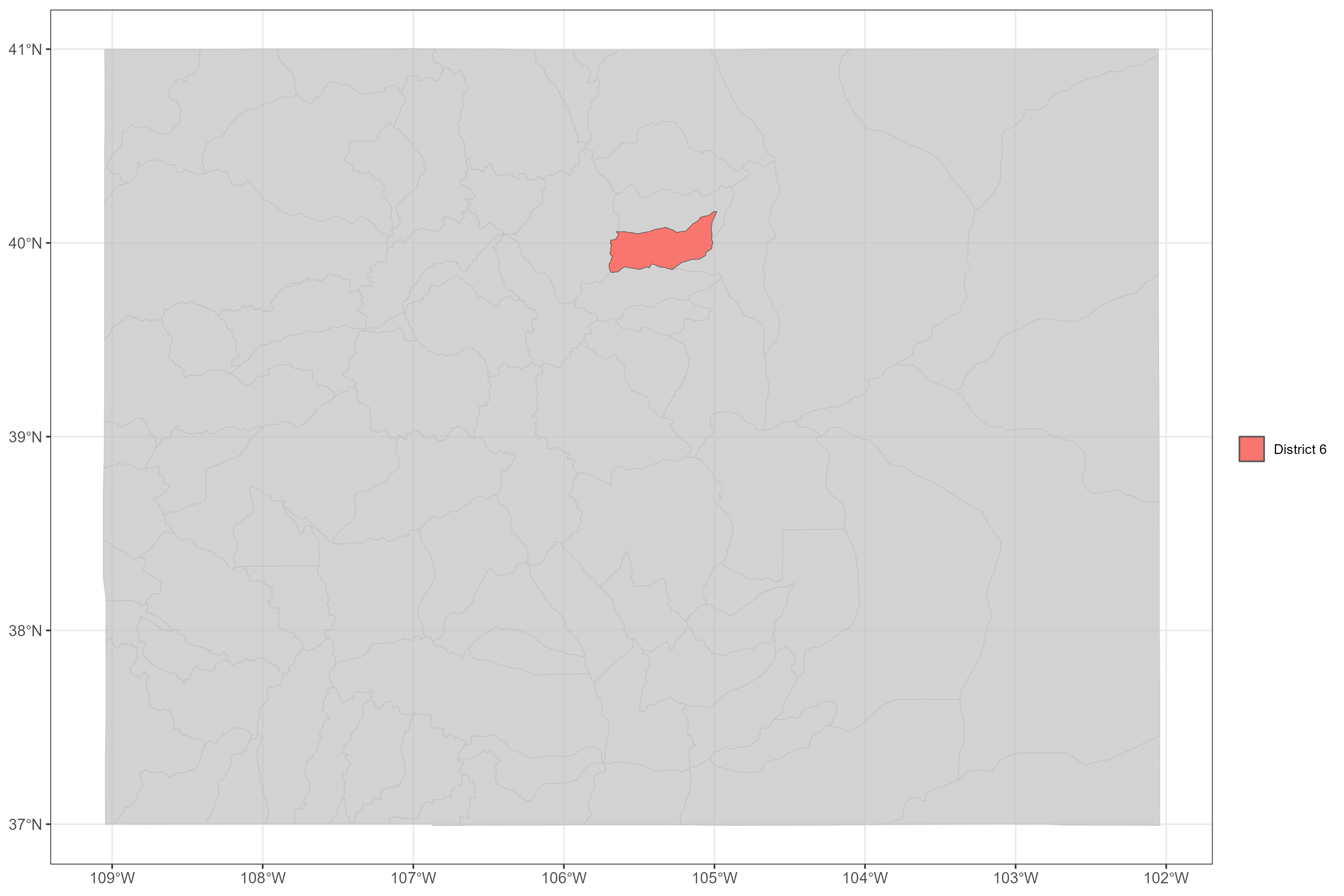
We loop through each one of the water districts and apply the same data collection process for each water district. For this example, we will walk through the data collection process for a single district, district 6.
# subset to example district 6
aoi <-
  districts %>%
  dplyr::filter(district == 6) %>%
  dplyr::select(district, division, basin, name, geometry)

aoi
#> Simple feature collection with 1 feature and 4 fields
#> Geometry type: POLYGON
#> Dimension:     XY
#> Bounding box:  xmin: -105.7008 ymin: 39.84716 xmax: -104.9851 ymax: 40.16224
#> Geodetic CRS:  WGS 84
#> # A tibble: 1 × 5
#>   district division basin        name                                   geometry
#>      <int>    <int> <chr>        <chr>                             <POLYGON [°]>
#> 1 6 1 South Platte Boulder Creek ((-105.6478 40.05384, -105.6488 …Use NHDPlusTools First thing we do is we get NHDPlus flowlines for
each district like so:
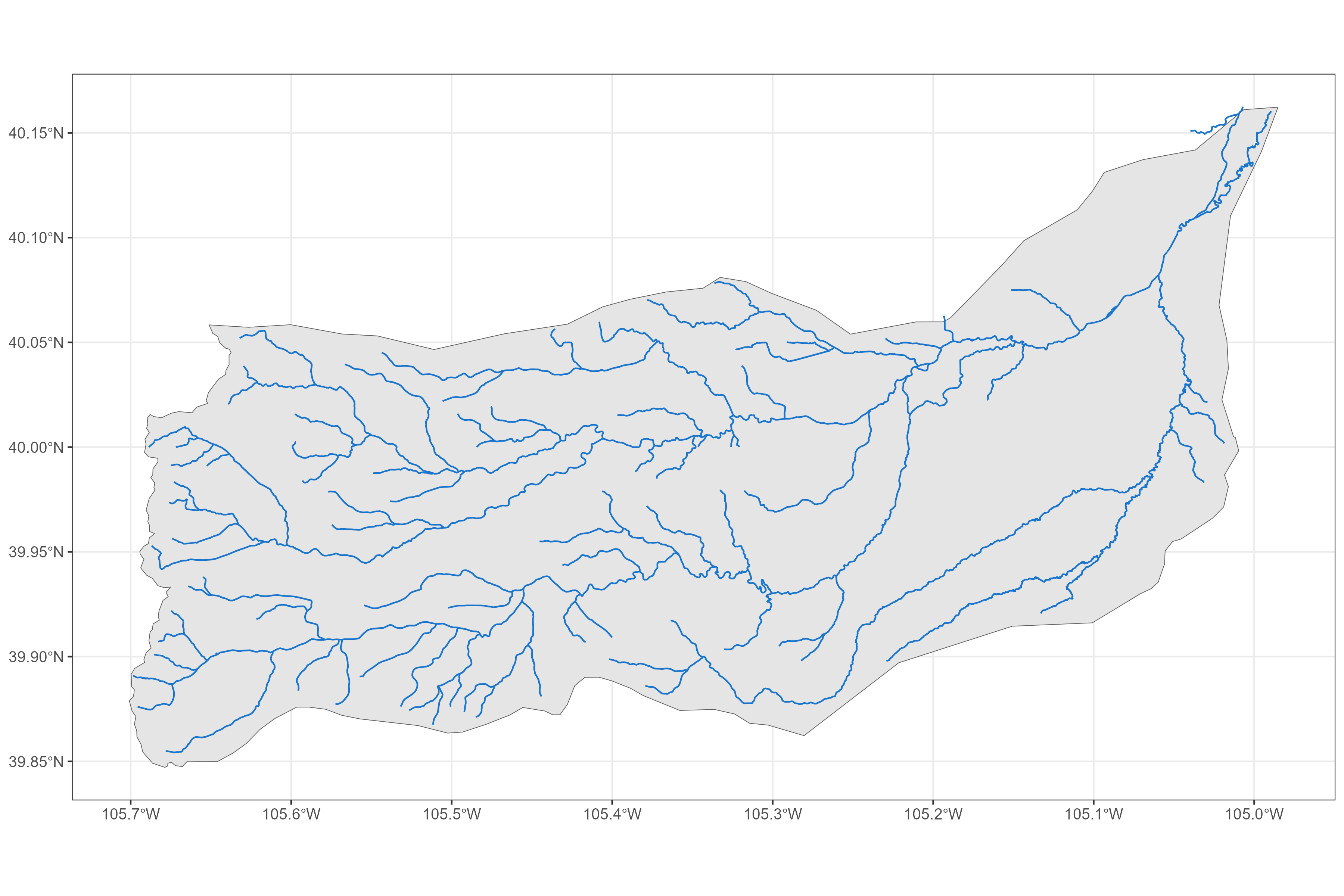
flowlines <- nhdplusTools::get_nhdplus(AOI = aoi)

nrow(flowlines)
#> [1] 327
We’ve got 327 unique flowlines in district 6.
By stream level
We remove any divergent flowlines (streamcalc != 0) and then get a list of all the unique streamlevels in our AOI. Below are the unique streamlevels in ascending order:
streamlevels <- sort(unique(dplyr::filter(flowlines, streamcalc != 0)$streamleve))We then select the top 2 largest streamlevels in our AOI
streamlevels <- streamlevels[1:3]
streamlevels
#> [1] 4 5 6
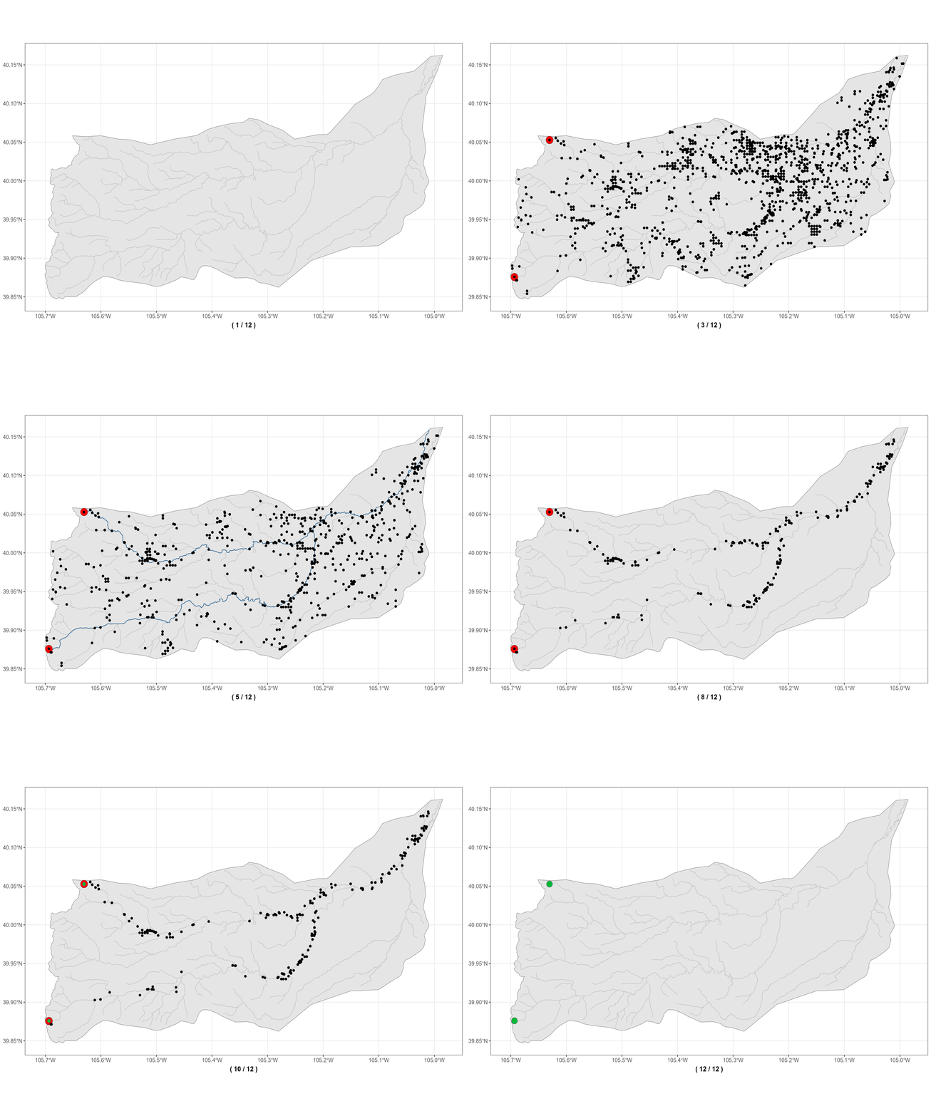
We then make sure to filter out any extraneous flowlines that are outside the bounds of the AOI. We are then left with the top 3 most promiment flowlines by streamlevel in our particular district of interest. From each streamlevel, we then found the most downstream flowline on that streamlevel by using the minimum Hydroseq attribute. We then navigate up the river network, following the mainstem of the river and find the most upstream flowline along the mainstem. The most upstream flowline along the mainstem path of each streamlevel will end up being the points we will use to decide which water rights (WDIDs) we will select for each district. This process is illustrated in the gif below.
Now that we have identified the mainstems within our AOI, and the most
upstream flowlines of these mainstems, we can use these upstream points
to identify the water rights we want to select for each district. First
we’ll get all the relevant water rights for the district, and remove any
missing data, removing data whose water_source is “GROUNDWATER”, and
applying a spatial filter to just points within 500 meters of a mainstem
river.
# get water rights information around most upstream of mainstems
water_rights <- cdssr::get_water_rights_netamount(
              water_district = "6"
              )

pts <-
  water_rights %>%
  dplyr::tibble() %>%
  dplyr::mutate(
    lon     = longitude,
    lat     = latitude,
    gnis_id = sub("^0+", "", gnis_id)
  ) %>%
  # dplyr::filter(wdid == "0604255") %>%
  dplyr::filter(!is.na(longitude) | !is.na(latitude)) %>%
  sf::st_as_sf(coords = c("longitude", "latitude"), crs = 4326) %>%
  sf::st_filter(aoi) %>%
  dplyr::filter(!grepl("GROUNDWATER", water_source)) %>%
  sf::st_filter(
  sf::st_transform(
      sf::st_buffer(
        sf::st_union(mainstems), 500),
      4326
      )
  )

dplyr::select(pts, water_district, wdid, structure_type, water_source, gnis_id, appropriation_date)
#> Simple feature collection with 802 features and 6 fields
#> Geometry type: POINT
#> Dimension:     XY
#> Bounding box:  xmin: -105.6933 ymin: 39.87131 xmax: -105.0106 ymax: 40.14638
#> Geodetic CRS:  WGS 84
#> # A tibble: 802 × 7
#>    water_district wdid    structure_type water_source gnis_id appropriation_date
#>             <int> <chr>   <chr>          <chr>        <chr>   <chr>
#>  1              6 0600501 Ditch          BOULDER CRE… 178354  1860-10-01 00:00:…
#>  2              6 0600501 Ditch          BOULDER CRE… 178354  1904-11-04 00:00:…
#>  3              6 0600501 Ditch          BOULDER CRE… 178354  1922-11-29 00:00:…
#>  4              6 0600501 Ditch          BOULDER CRE… 178354  1929-12-31 00:00:…
#>  5              6 0600501 Ditch          BOULDER CRE… 178354  1935-11-30 00:00:…
#>  6              6 0600502 Ditch          BOULDER CRE… 178354  1922-11-10 00:00:…
#>  7              6 0600503 Ditch          BOULDER CRE… 178354  1922-11-10 00:00:…
#>  8              6 0600504 Ditch          BOULDER CRE… 178354  1922-11-10 00:00:…
#>  9              6 0600505 Ditch          BOULDER CRE… 178354  1922-11-10 00:00:…
#> 10              6 0600506 Ditch          BOULDER CRE… 178354  1922-11-10 00:00:…
#> # ℹ 792 more rows
#> # ℹ 1 more variable: geometry <POINT [°]>
After subsetting our data, we have 802 unique water rights, which correspond to 236 unique WDID locations
length(unique(pts$wdid))
#> [1] 236
We then identify the indices of the points nearest to most upstream flowline, and thus we’ve found the most upstream WDIDs along our mainstem flowlines.
# GET index of nearest points to each uppermost flowline
near_idx <- unique(
              unlist(
                lapply(1:nrow(upstream_fline), function(z) {

                  sf::st_nearest_feature(
                    sf::st_transform(upstream_fline[z, ], 4326),
                    pts
                    )
                  })
                )
              )

# WDIDs of interest
pts[near_idx, ] %>%
  sf::st_drop_geometry() %>%
  dplyr::select(water_district, wdid, structure_type, water_source, gnis_id, appropriation_date)
#> # A tibble: 2 × 6
#>   water_district wdid    structure_type water_source  gnis_id appropriation_date
#>            <int> <chr>   <chr>          <chr>         <chr>   <chr>
#> 1              6 0604256 Reservoir      NORTH BOULDE… 178467  1907-10-03 00:00:…
#> 2              6 0602105 Reservoir      SOUTH BOULDE… 180974  1976-03-17 00:00:…
The gif below walks through the process described above for finding the most upstream WDIDs for each of our mainstem flowlines in the district of interest:
Subset the water rights by river and determine which water right should be associated with each mainstems most upstream point.
We then will do some fuzzy string matching to subset the water rights points down to the same GNIS ID of our most upstream flow line points (red points above). Now we only have points that match the same GNIS ID of our upstream points, the next step we take is to find the nearest neighboring water right point to each of our upstream mainstem flowlines.
To recap: For each district, we get the biggest river(s), find the most upstream point(s), and then find a water right(s) that represents the most upstream point(s) on each mainstem.
Techniques used:
- fuzzy string matching
- basic
distance/nearest neighbor calculation
Now we have selected the WDIDs we will be using for our district of
interest/AOI. We can use thecdssr package to get water right call
data
for each of our selected water rights in our district of interest/AOI.
The CDSS REST API provides an analysis service that allows you to provide a WDID and an admin number and request a call analysis that returns a time series showing the percentage of each day that the specified WDID and priority was out of priority and the downstream call in priority.
Given this information we decided to prescribe a “99999.00000” to each of our upstream WDIDs, such that each of these WDID water right locations is now representing the most junior water right possible. simulate the experience of an extremely junior rights holder, located as far upstream as possible (i.e. what it would be like if you were at the top of the river and you had no water rights –> all downstream users get first dibs on water)
Here we use cdssr to get call analysis data for each of WDIDs of
interest
# get call data for WDID "0604256"
calls <- cdssr::get_call_analysis_wdid(
  wdid       = "0604256",
  admin_no   = "99999.00000",
  start_date = "1970-01-01",
  end_date   = "2023-01-01"
)

calls <-
  calls %>%
  dplyr::select(datetime,
         wdid        = analysis_wdid,
         priority_date,
         out_pct     = analysis_out_of_priority_percent_of_day
         )
head(calls)
#>     datetime    wdid priority_date out_pct
#> 1 1970-01-01 0604256          <NA>       0
#> 2 1970-01-02 0604256          <NA>       0
#> 3 1970-01-03 0604256          <NA>       0
#> 4 1970-01-04 0604256          <NA>       0
#> 5 1970-01-05 0604256          <NA>       0
#> 6 1970-01-06 0604256          <NA>       0
The call anaylsis by WDID tool from CDSS, allows us to gather a daily timeseries for each of the WDIDs we selected in each district.
The percent out of priotity timeseries provides 2 key data points that we used for our analysis: 1. Daily out of priority percentage 2. The water right date of the downstream water right that calls out junior upstream users.
For each daily timestamp, we wanted to determine the most senior right that would call out of super junior upstream WDID of interest for each mainstem in each district. For each of our WDIDs that we collected call out data for, we calculated an annual average call year which indicates for a given mainstem river and a given year, what the average water right call year was for that mainstem/year.


