Linear-Program-Solvers
Introduction
- This repository contains implementations of following linear program (LP) solver algorithms in Python and NumPy:
- Simplex algorithm
- Primal-Dual Infeasible Interior Point method
- Brute force algorithm (exhaustive search over all possible bases)
- The solvers are tested on concrete max-flow (network flow) problems (see Results section below)
- Refer to in-code documentation and comments for description of how the code is working
Repository structure
- Directory
solvers/contains the implementation of the mentioned solvers- Implementation of
SimplexSolverclass can be found insolvers/simplex_solver.py - Implementation of
InteriorPointSolverclass can be found insolvers/interior_point_solver.py - Implementation of
BruteSolverclass can be found insolvers/brute_solver.py
- Implementation of
utils.pycontains definition of the following useful helper functions:network_flow_to_std_LP()that converts a given max-flow problem instance to its corresponding LPprimal_to_dual()that converts a given primal LP in standard form to its corresponding dual in standard form
main.pycontains example driver code that solves two max-flow problem instances using the solvers
Results
We test SimplexSolver and InteriorPointSolver on two separate max-flow instances.
-
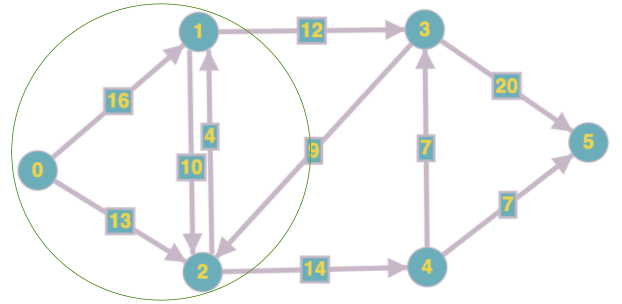
Network for first max-flow instance is given below (green circle marks a min-cut of the network)

SimplexSolvergives the following flow assignment for this instance:
| Edge | Flow | Capacity |
|---|---|---|
| (0, 1) | 16 | 16 |
| (0, 2) | 10 | 13 |
| (1, 2) | 8 | 10 |
| (1, 3) | 12 | 12 |
| (2, 1) | 4 | 4 |
| (2, 4) | 14 | 14 |
| (3, 2) | 0 | 9 |
| (3, 5) | 19 | 20 |
| (4, 3) | 7 | 7 |
| (4, 5) | 7 | 7 |
The total flow leaving source (vertex-0) in the above flow assignment (16 + 10 = 26) is equal to the sum of the capacities of edges going out of the cut shown above in green (12 + 14 = 26). Hence, this flow assignment is optimal (cf. max-flow min-cut theorem)
-
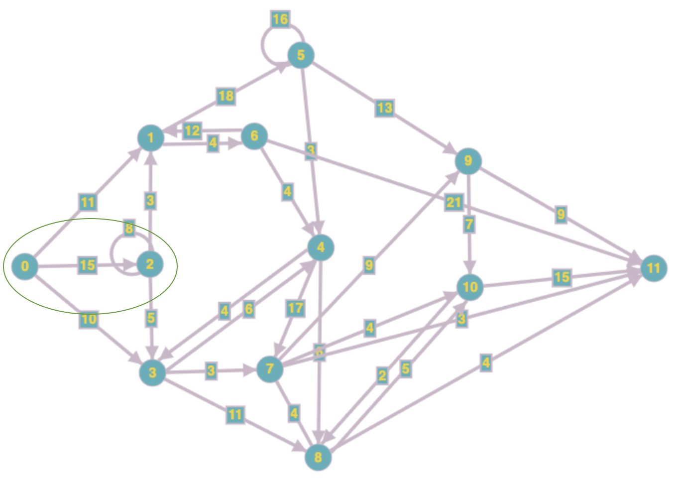
Network for second max-flow instance is given below (green circle marks a min-cut of the network)

InteriorPointSolvergives the following flow assignment for this instance:
| Edge | Flow | Capacity |
|---|---|---|
| ( 0, 1) | 11.00 | 11 |
| ( 0, 2) | 8.00 | 15 |
| ( 0, 3) | 10.00 | 10 |
| ( 1, 5) | 11.09 | 18 |
| ( 1, 6) | 3.48 | 4 |
| ( 2, 1) | 3.00 | 3 |
| ( 2, 2) | 4.00 | 8 |
| ( 2, 3) | 5.00 | 5 |
| ( 3, 4) | 5.17 | 6 |
| ( 3, 7) | 2.27 | 3 |
| ( 3, 8) | 8.33 | 11 |
| ( 4, 3) | 0.76 | 4 |
| ( 4, 7) | 5.72 | 17 |
| ( 4, 8) | 1.05 | 6 |
| ( 5, 4) | 1.76 | 3 |
| ( 5, 5) | 8.00 | 16 |
| ( 5, 9) | 9.33 | 13 |
| ( 6, 1) | 0.58 | 12 |
| ( 6, 4) | 0.61 | 4 |
| ( 6, 11) | 2.30 | 21 |
| ( 7, 8) | 1.00 | 4 |
| ( 7, 9) | 4.64 | 9 |
| ( 7, 10) | 3.02 | 4 |
| ( 7, 11) | 2.33 | 3 |
| ( 8, 7) | 3.00 | 4 |
| ( 8, 10) | 4.37 | 5 |
| ( 8, 11) | 3.50 | 4 |
| ( 9, 10) | 5.83 | 7 |
| ( 9, 11) | 8.14 | 9 |
| (10, 8) | 0.49 | 2 |
| (10, 11) | 12.73 | 15 |
The total flow leaving source (vertex-0) in the above flow assignment (11 + 8 + 10 = 29) is equal to the sum of the capacities of edges going out of the cut shown above in green (11 + 3 + 5 + 10 = 29). Hence, this flow assignment is optimal (cf. max-flow min-cut theorem)
References
- Introduction to Linear Optimization by Dimitris Bertsimas, John Tsitsiklis
- Interior-Point Methods by Stephen Wright