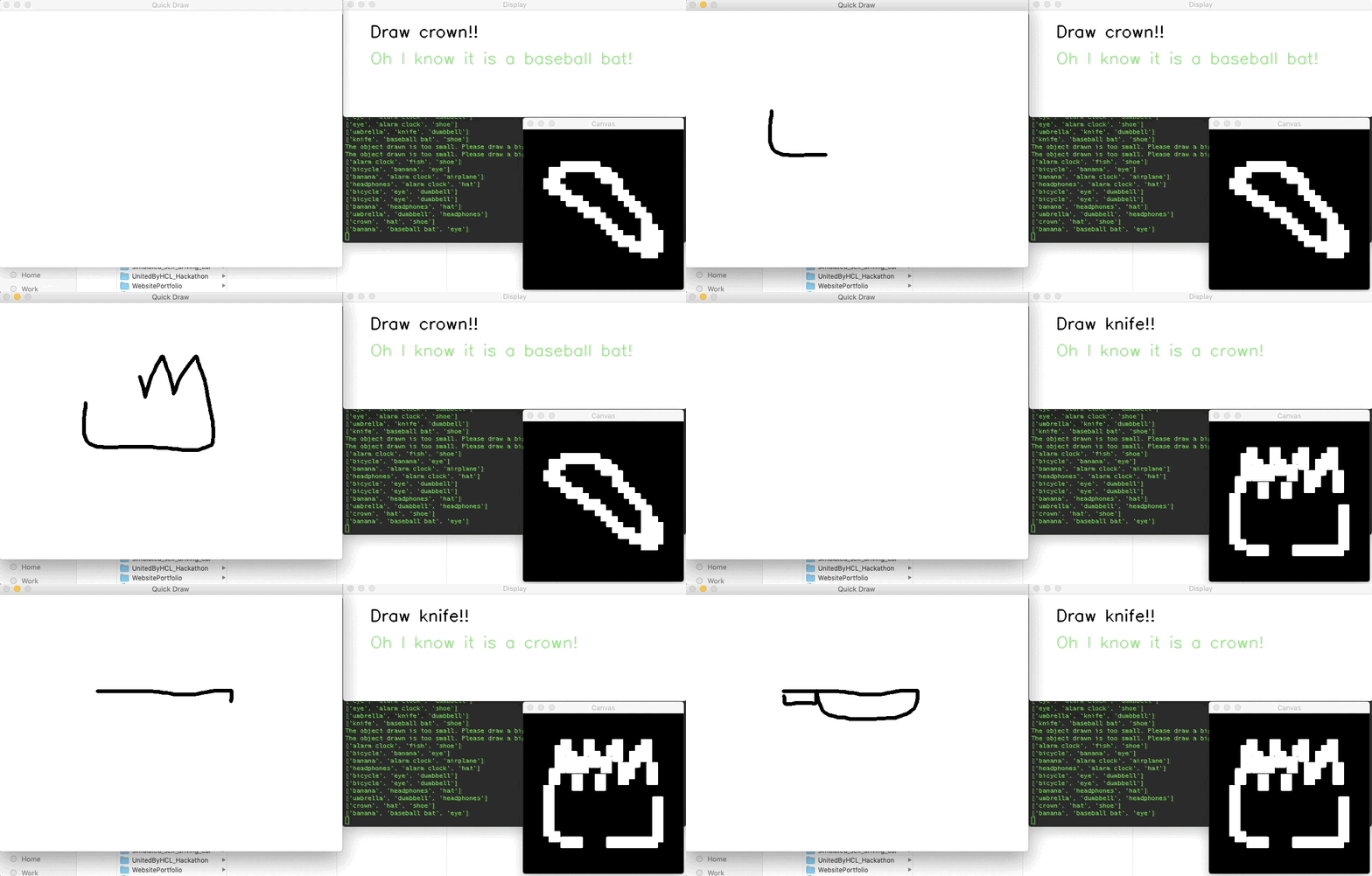
This project is done as a part of Computer Vision Course.
In Quick Draw the AI system tries to classify the hand-drawn doodle into a predetermined category. By this project we are trying to achieve the same using different feature extraction techniques like HOG, LBP, SIFT, SURF, pixel values with feature reduction techniques PCA, LDA and applying various classifiers such as Naive Bayes, Random Forest, SVM, XGBoost, Bagging, ADA-boost, KNN and CNN to compare their performance on different evaluation metric such as Accuracy, MAP@3, CMC Curve and Confusion Matrix.
Project Poster can be found in CV-Poster-Final.pdf.
- It is a challenge in Computer Vision & Machine Learning to handle noisy data and dataset with many different representations of the same class. The Quick Draw Doodle Recognition challenge is a good example of these issues because different users may draw the same object differently or the doodles could be incomplete which is similar to noisy data.
- This application can be used as a fast prototyping tool for designers or artists by suggesting them the accurate templates on the basis of the rough doodles made by them.
- It can be extended by replacing the doodles with doodles of alphabets and then convert the hand-written text into digital text format.
- The Quick Draw dataset is a collection of millions of doodle drawings of 300+ categories. The drawings draw by the players were captured as 28 x 28 grayscale images in .npy format with respect to each category.
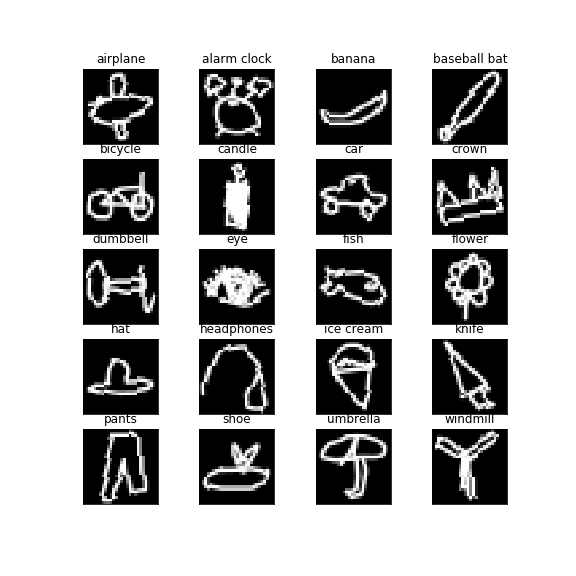
- The complete dataset is huge (~73GB) and so we have used only a subset of the complete data (20 categories).
- The dataset is split in training and test set with 80-20 ratio, the training set is further split into train and validation with 70-30 ratio.
- Fig above shows a doodle image of each class in our sampled dataset.
- Dataset can be downloaded from here.
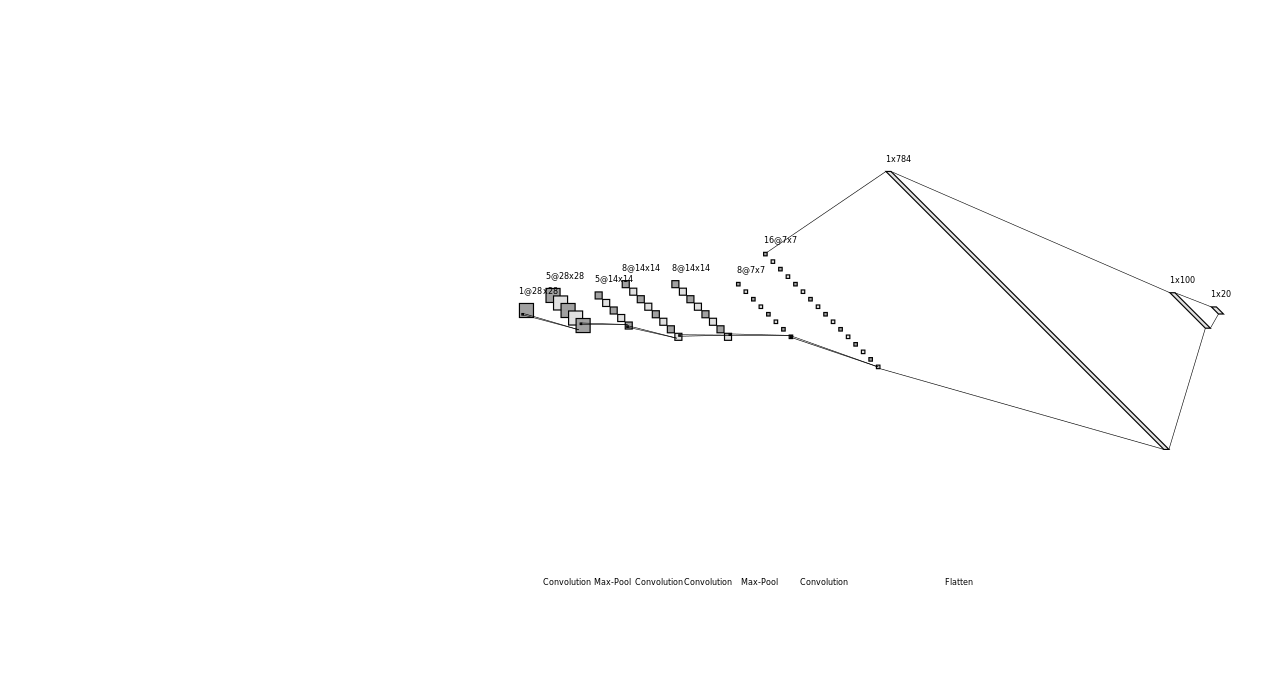
- CNN Model Architecture
-
We have followed a conventional computer vision pipeline to train our model. Fig. below shows the training pipeline followed.
-
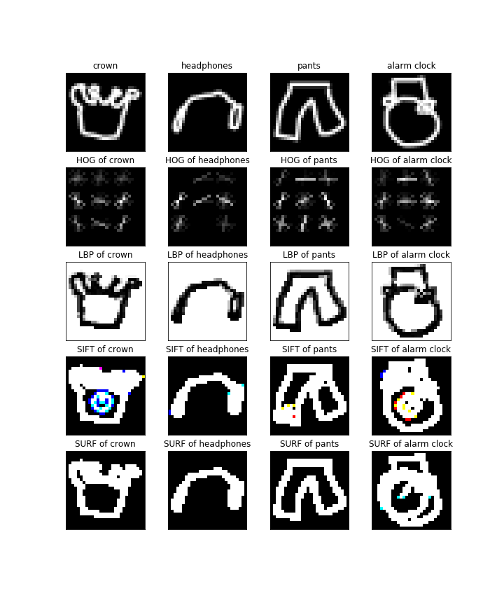
Feature Extraction: Extract texture information from HOG & LBP, Spatial information from SIFT & SURF and pixel information from grayscale image.
-
Preprocessing: Feature normalization by Min-Max and Z-score to bring features on a similar scale.
-
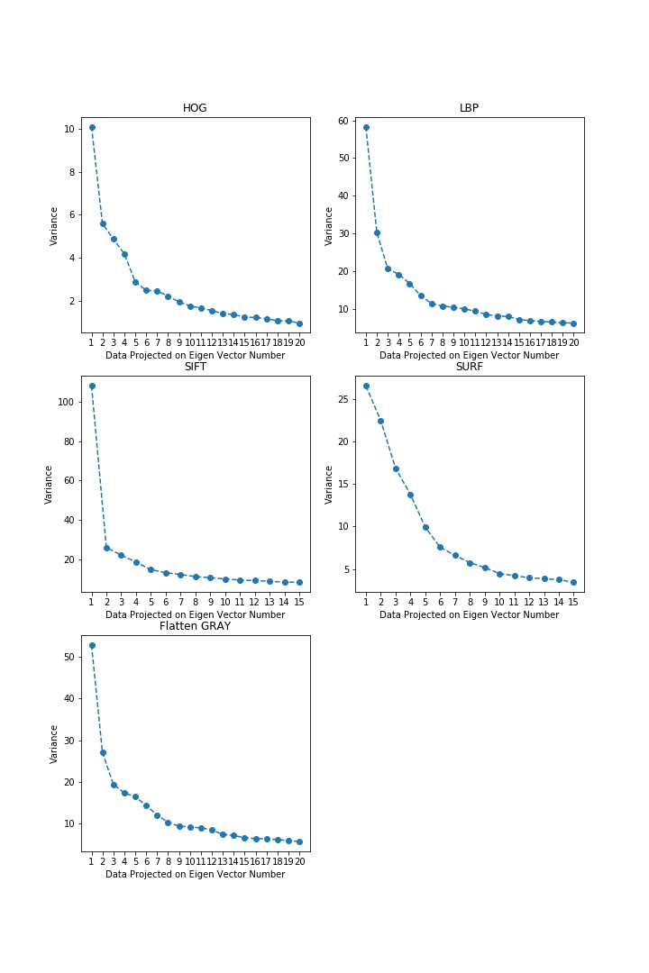
Dimensionality Reduction: PCA or LDA was applied to project the features with max separation. In PCA number of components were selected by plotting the variance over projected data.
-
Classification: Different classifiers were trained and tested with different parameters and feature combinations.
-
Prediction and Evaluation Metrics: Metrics such as accuracy, MAP@3, CMC curve was found to compare the performance of classifiers.
-
For Production time the following pipeline was used where contours were used to find the object.
Follwing are the results of the project:
-
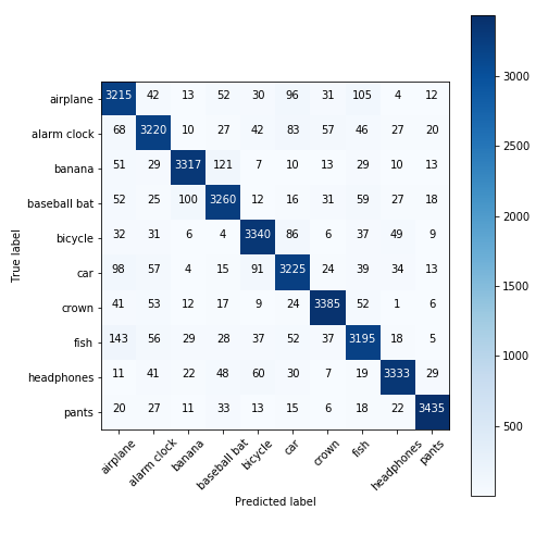
Confusion Matrices were plotted for best performing classifiers.
-
Mean Average Precision (MAP@3) score were found for classifiers to find performance in top 3 predictions.
-
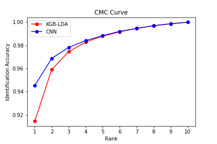
CMC Curve was plotted to find the identification accuracy at different ranks.
-
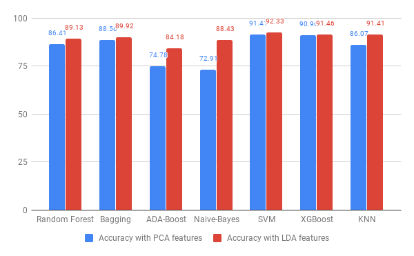
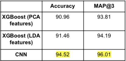
Accuracy of different classifiers was used to compare the performance using PCA and LDA.
- In Dimensionality reduction technique LDA performs better than PCA as it is able to separate data on the basis of classes.
- Texture based features gave good classification accuracy as compared to other features.
- XGBoost shows best performance as compared to all the other non-deep learning models as the dataset includes images of multiple classes over which XGboost is able to learn better because of boosting technique.
- CNN gives the best performance with a MAP@3 of 96.01%. This is because the kernels are able to learn different feature representations which help the model to differentiate between the classes well.
- Lu, W., & Tran, E. (2017). Free-hand Sketch Recognition Classification.
- M. Eitz, J. Hays, and M. Alexa. How do humans sketch objects? ACM Trans. Graph. (Proc. SIGGRAPH), 31(4):44:1– 44:10, 2012.
- K. He, X. Zhang, S. Ren, and J. Sun. Deep residual learning for image recognition. IEEE Conference on Computer Vision and Pattern Recognition, 2016.
- Kim, J., Kim, B. S., & Savarese, S. (2012). Comparing image classification methods: K-nearest-neighbor and support-vector machines. Ann Arbor, 1001, 48109-2122.
- Ha, D., & Eck, D. (2017). A neural representation of sketch drawings. arXiv preprint arXiv:1704.03477.
- Anubhav Shrimal
- Vrutti Patel
