FaultSeg3D: using synthetic datasets to train an end-to-end convolutional neural network for 3D seismic fault segmentation
This is a Keras version of FaultSeg implemented by Xinming Wu for 3D fault segmentation
As described in FaultSeg: using synthetic datasets to train an end-to-end convolutional neural network for 3D fault segmentation by Xinming Wu1, Luming Liang2, Yunzhi Shi1 and Sergey Fomel1. 1BEG, UT Austin; 2Uber.
If you would just like to try out a pretrained example model, then you can download the pretrained model and use the 'prediction.ipynb' script to run a demo.
To train our CNN network, we automatically created 200 pairs of synthetic seismic and corresponding fault volumes, which were shown to be sufficient to train a good fault segmentation network.
The training and validation datasets can be downloaded here
Run train3 to start training a new faultSeg model by using the 200 synthetic datasets
If you find this work helpful in your research, please cite:
@article{wu2019faultSeg,
    author = {Xinming Wu and Luming Liang and Yunzhi Shi and Sergey Fomel},
    title = {Fault{S}eg3{D}: using synthetic datasets to train an end-to-end convolutional neural network for 3{D} seismic fault segmentation},
    journal = {GEOPHYSICS},
    volume = {84},
    number = {3},
    pages = {IM35-IM45},
    year = {2019},
}
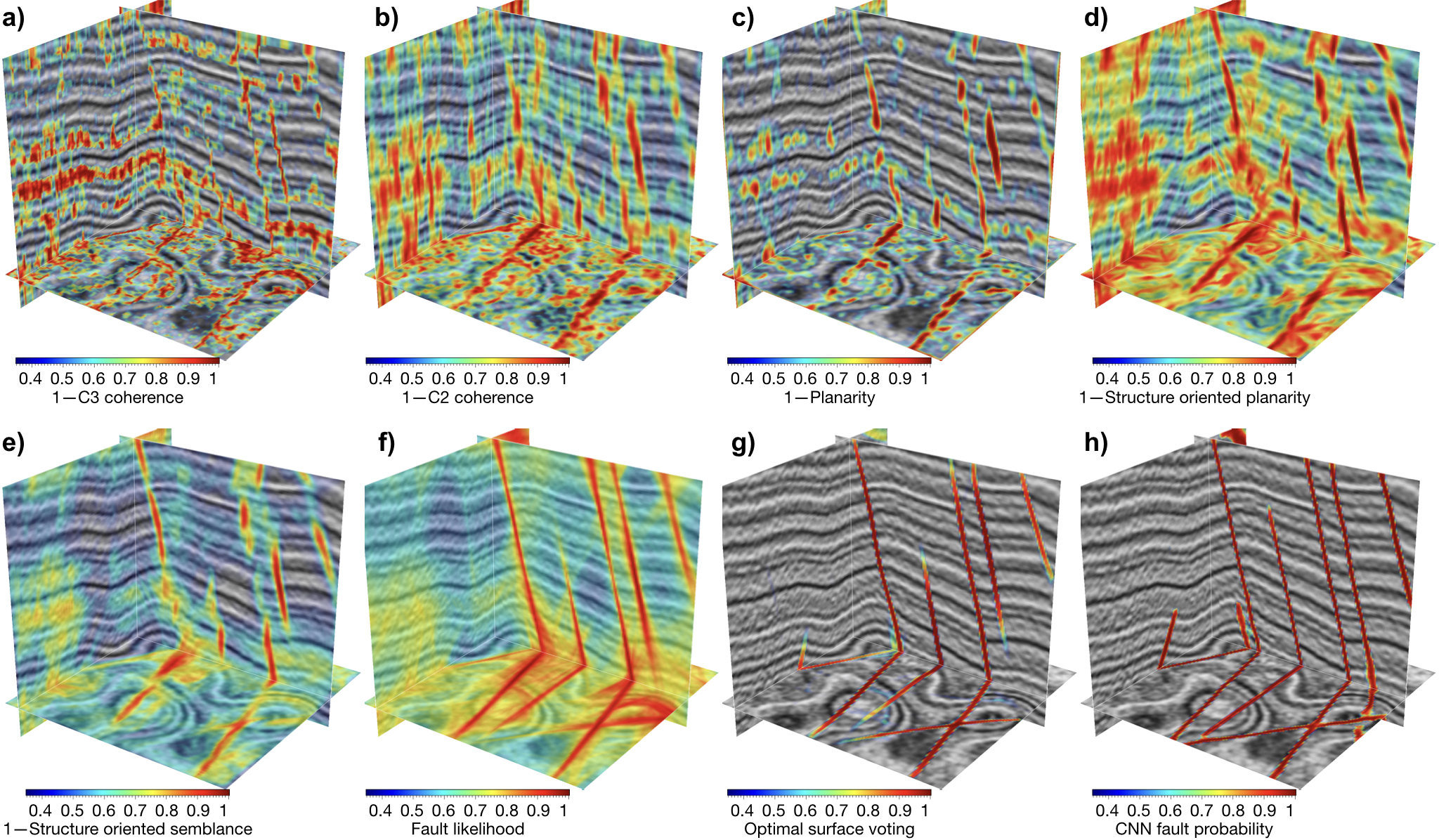
Fault detections are computed on a syntehtic seismic image by using 8 methods of C3 (Gersztenkorn and Marfurt, 1999),
C2 (Marfurt et al., 1999), planarity (Hale, 2009), structure-oriented linearity (Wu, 2017), structure-oriented semblance (Hale, 2009), fault likelihood (Hale, 2013; Wu and Hale, 2016, code), optimal surface voting (Wu and Fomel, 2018, code) and our CNN-based segmentation.
To quantitatively evaluate the fault detection methods, we further calculate the precision-recall (Martin et al., 2004) and receiver operator characteristic (ROC) (Provost et al., 1998) curves shown below. From the precision-recall curves, we can clearly observe that our CNN method (red curve) provides the highest precisions for all the choices of recall.

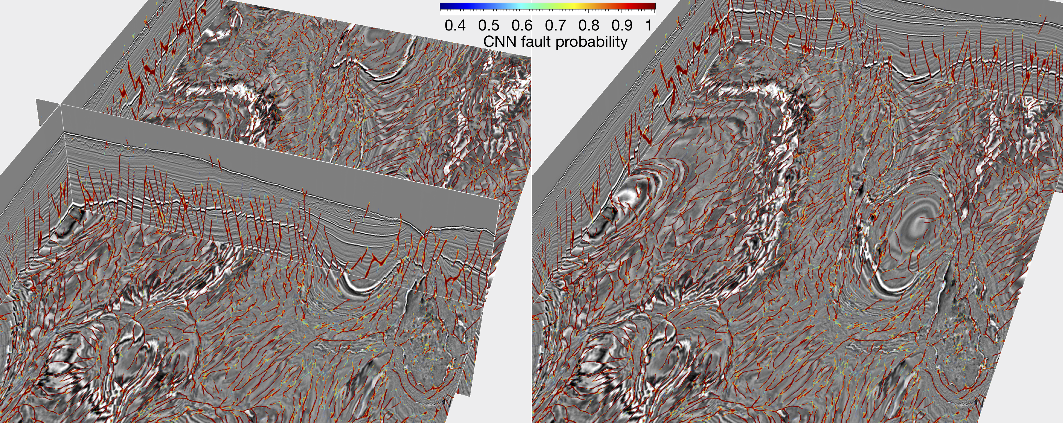
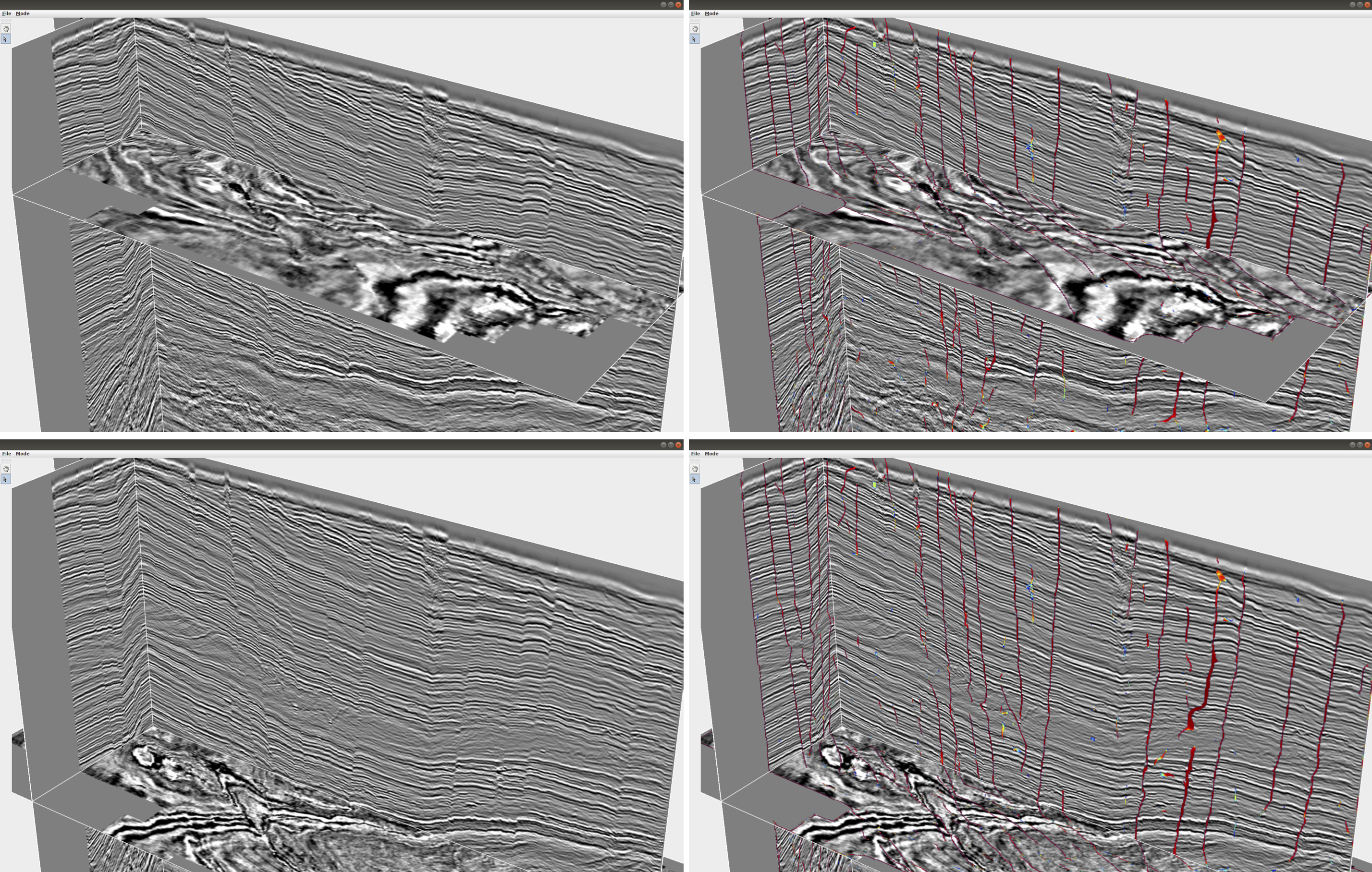
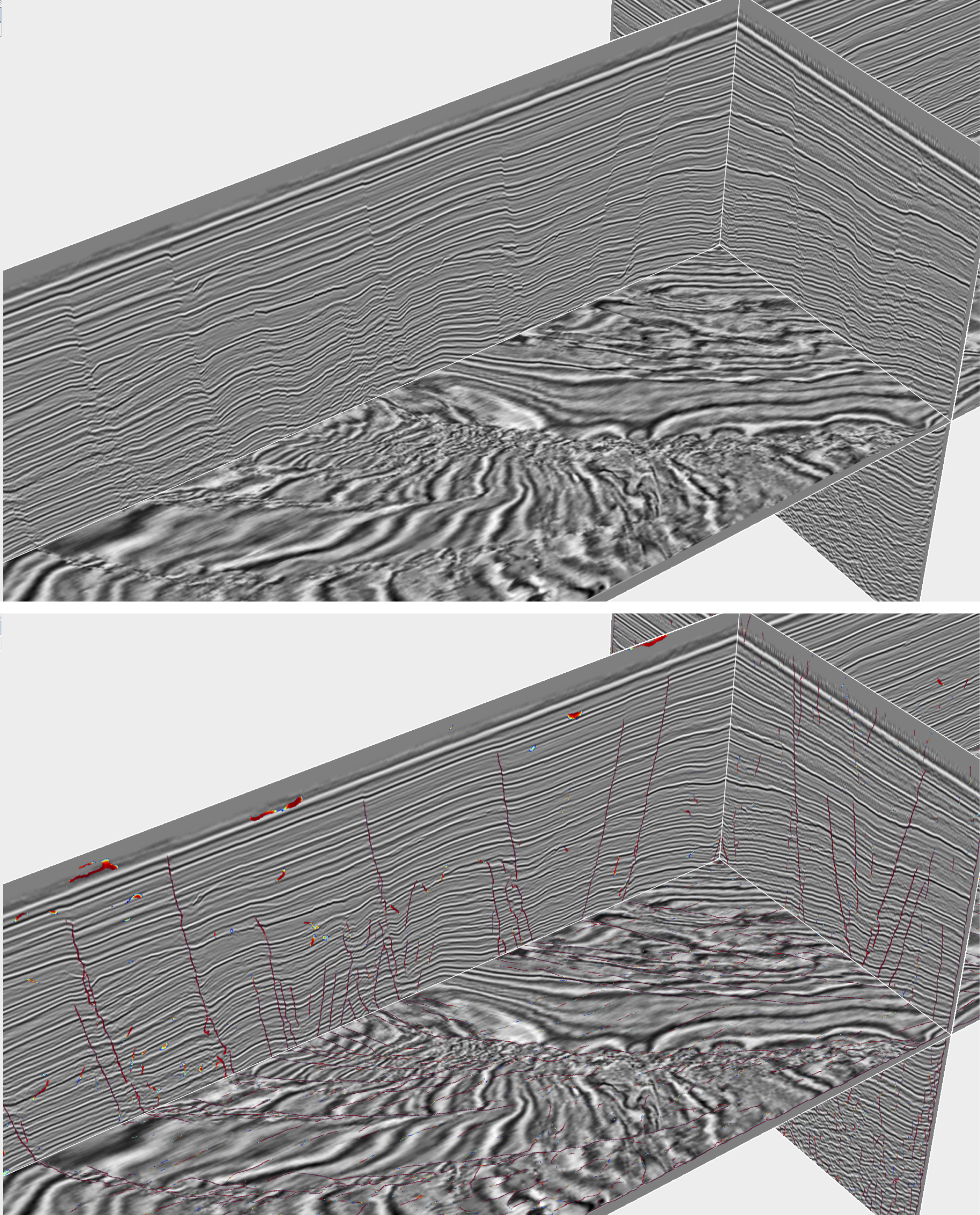
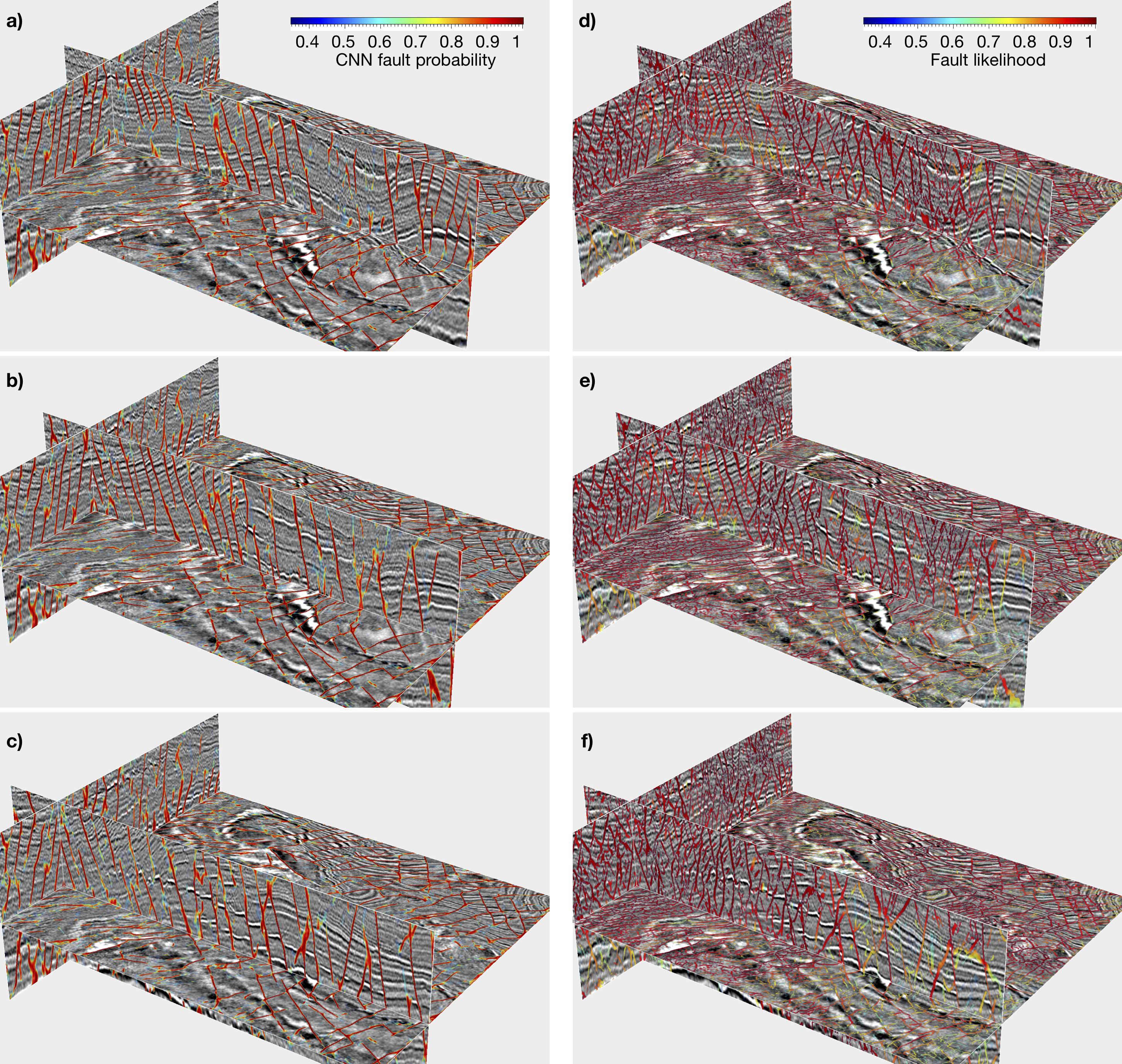
Although trained by only synthetic datasets, the CNN model works well in predicting faults in field datasets that are acquired at totally different surveys.
Example of Netherlands off-shore F3 (provided by the Dutch Government through TNO and dGB Earth Sciences)
compare the CNN fault probability (top right) with fault likelihood (bottom)
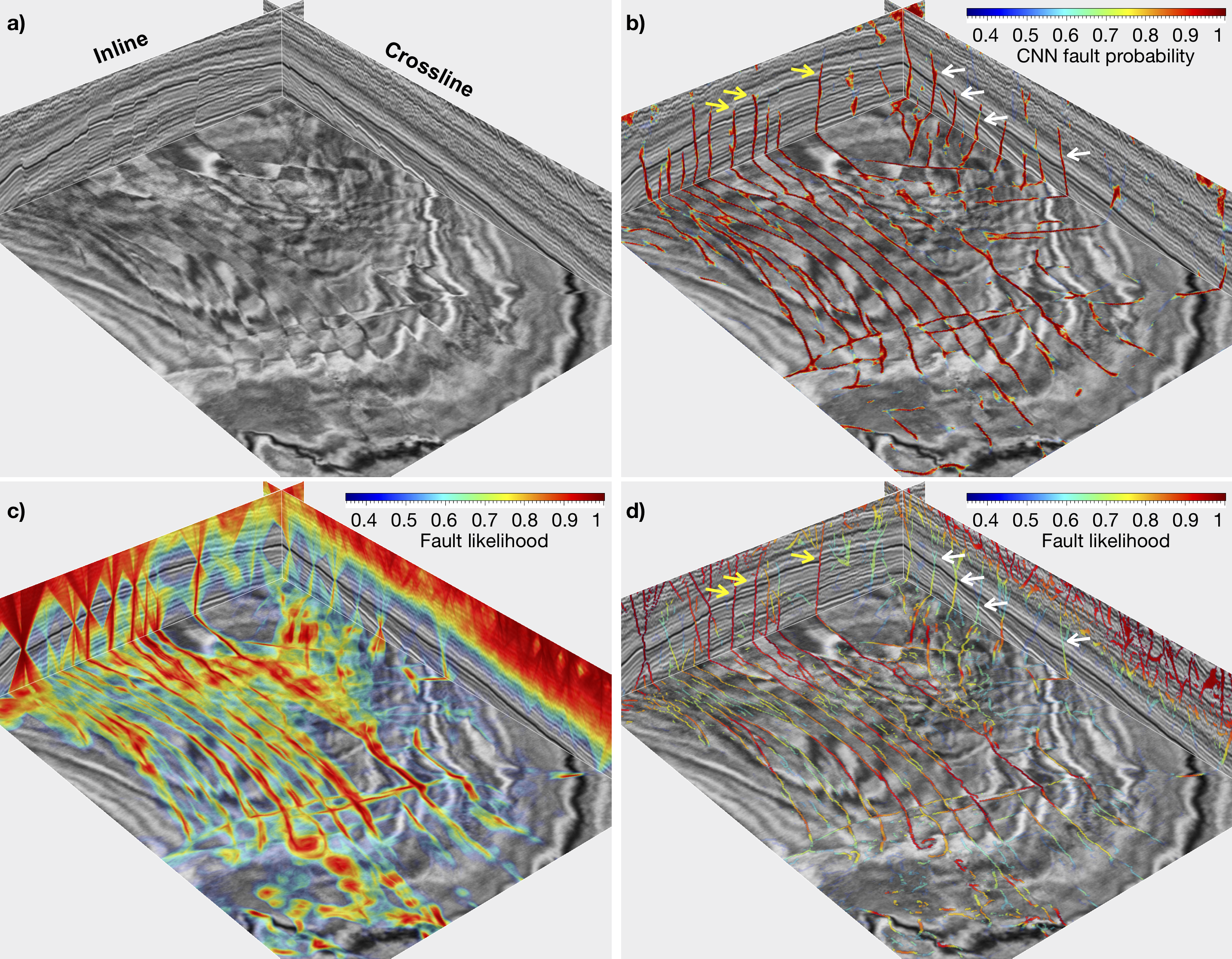
compare the CNN fault probability (middle) with fault likelihood (right)

Example of Costa Rica (acquired in the subduction zone, Costa Rica Margin, provided by Nathan Bangs)
compare the CNN fault probability (left column) with fault likelihood (right column)
Example of Kerry-3D (The fault features have been thinned in this example)
Example of Opunake-3D (The fault features have been thinned in this example)
This extension to the Keras library is released under a creative commons license which allows for personal and research use only. For a commercial license please contact the authors. You can view a license summary here: http://creativecommons.org/licenses/by-nc/4.0/
