aobject/NYU-AI-Project-02

NYU-AI-Project-02

NYU // AI // Project 02 // Continuous Learning

This repository and project was developed for the CS-GY-6613 Artificial Intelligence class at NYU. The class professor is Pantelis Monogioudis. The Teacher’s Assistants are Shalaka Sane and Zhihao Zhang. They have our deep graditude for all guidance they offered in the development of the project.

We would also like to thank Vincenzo Lomonaco, one of the creators of the CORe50 dataset. He generously answered our questions and provided great advice.

The authors of the project are Justin Snider and Jason Woo.

Using Rehearsal and Elastic Weight Consolidation for Single-Incremental-Task on New Classes

This project implements a series of continuous learning strategies using the CORe50 dataset. We have focused on implementing Rehearsal, Elastic Weight, and finally a hybrid of two strategies combined. We will explain the logic, implementation, and performance of these three strategies.

Continual Learning

The recognition of object class types through sensor data such as pixels has important application. Machine Learning algorithms have shown themselves very capable at learning individual task. The more focused the higher the performance. However, for a more generalized artificial intelligence agent to be affective it will need to learn many tasks, not just one.

Continual Learning is an area of artificial intelligence research focused on the challenge of learning multiple task.

There are several impediments to continual learning. Beyond the general limitations of computer hardware, we find that machine learning networks suffer from a problem called Catastrophic Forgetting.

Single-Incremental-Tasks (SIT) is the challenge to take on different tasks. New Classes (NC) is a subcategory of SIT. For a New Classes we challenge the algorithm to learn disjoint tasks. For example our goal might be to identify if the class is present in a given image.

Many strategies have been developed to combat catastrophic forgetting. The three types of strategies are architectural, regularization and rehearsal. In this project, we focus on elastic weight consolidation (EWC), a regularization strategy, and a custom implementation of a rehearsal strategy. We also combine the two. A diagram of different types of specific CL implementations is shown below.

Different Continuous Learning Strategies

Figure from [1].

CORe50 Dataset

Image from [4].

Dataset Description

There are few available data sets that are suitable for evaluating techniques that are meant to tackle single incremental task (SIT) learning . CORe50 is an image based data set which is specifically designed to evaluate CL techniques.

CORe50, specifically designed for (C)ontinual (O)bject (Re)cognition, is a collection of 50 domestic objects belonging to 10 categories: plug adapters, mobile phones, scissors, light bulbs, cans, glasses, balls, markers, cups and remote controls. Classification can be performed at object level (50 classes) or at category level (10 classes).

The full dataset consists of 164,866 128×128 RGB-D images: 11 sessions × 50 objects × (around 300) frames per session. Three of the eleven sessions (#3, #7 and #10) have been selected for test and the remaining 8 sessions are used for training.

The code for for loading the data set is freely available and the link to the github is provided here.

Example Images

Object 1	Object 2	Object 3

Rehearsal

A very simple approach to solving CL problems is rehearsal. In rehearsal, data from previous tasks is periodically appended to the training data for a new task. The goal of rehearsal is to "strengthen the connection for memories [the model] has already learned." While this approach seems simple, the practicality of it is limited.

Some of the challenges we faced was computation and storage abilities. Given our ability to run the model only on our local machines, we found that appending all of the previous tasks data into the training of a new task was unfeasible. To accommodate this, only half of the previous tasks' data was used.

Modifications to the provided naive_baseline.py

for i, train_batch in enumerate(dataset):
    train_x, train_y, t = train_batch

    # Start modification

    # run batch 0 and 1. Then break. 
    # if i == 2: break

    # shuffle new data
    train_x, train_y = shuffle_in_unison((train_x, train_y), seed=0)

    if i == 0: 
        # this is the first round
        # store data for later 
        all_x = train_x[0:train_x.shape[0]//2]
        all_y = train_y[0:train_y.shape[0]//2] 
    else: 
        # this is not the first round
        # create hybrid training set old and new data
        # shuffle old data
        all_x, all_y = shuffle_in_unison((all_x, all_y), seed=0)

        # create temp holder
        temp_x = train_x
        temp_y = train_y

        # set current variables to be used for training
        train_x = np.append(all_x, train_x, axis=0)
        train_y = np.append(all_y, train_y)
        train_x, train_y = shuffle_in_unison((train_x, train_y), seed=0)

        # append half of old and all of new data 
        temp_x, temp_y = shuffle_in_unison((temp_x, temp_y), seed=0)
        keep_old = (all_x.shape[0] // (i + 1)) * i
        keep_new = temp_x.shape[0] / q/ (i + 1)
        all_x = np.append(all_x[0:keep_old], temp_x[0:keep_new], axis=0)
        all_y = np.append(all_y[0:keep_old], temp_y[0:keep_new])
        del temp_x
        del temp_y

Rehearsal Parameters

Keeping too many old samples increases memory requirements and processing time, but allows better accuracy.

Here are the optimal hyperparameters.

Old Data Per Batch	New Data Per Batch
Equal proportion of all tasks retained to use for next round. About 11,990 old observations saved for use in next round throughout process.	About 11,990 new task observations used in each round.

Here are the pros and cons of changing the hyperparameters.

	Increase Observations	Decrease Observations
Pros	Increase in accuracy.	Increase in speed and efficiency.
Cons	High memory use and slow runtimes.	Decrease in performance.

Keeping less old samples uses less memory and processing time, but causes a decrease in accuracy.

Finding the sweet spot allows efficient use of memory and processing time. It also still provides much improved performance over the naive training model.

Accuracy Results using Rehearsal

Elastic Weight Consolidation

Regularization is the process of adding a penalty to the loss function to control the model from overfitting. In EWC, the loss function is extended with terms promoting selective consolidation of the weights which are important to retain past memories. Just as L2 regularization adds to the mean squared error for linear regression, EWC does something similar.

EWC is a regularization strategy in which the loss function as defined by [2].

is the loss for task B only.
is the Fisher Information Matrix.
can be considered as the importance of task A relative to task B.

This figure conceptually shows EWC moving weights into the intersection of low error for both task A and B. This differs from other techniques that just try to minimize the error for the new task, irrespective of the previous task.

Figure taken from [2].

EWC Parameters

Value too high causes the weights to favor previous learned tasks. So learning new tasks is slowed or prevented. This is because the elastic nature of the neural network that allows learning is slowed or stopped.

EWC Lambda	Analysis	Results
40.0	Too High	Learning was prevented by high penalty.
4.0	Ideal	Best combination of ability to learn new tasks and retain old tasks.
0.04	Too Low	Old tasks were forgotten very quickly.

EWC Implementation 01

Store a dictionary of fisher matrix values and optimum weights for every unique task. More effective at finding weights that work for multiple tasks. However, this requires more memory for every task to store the fisher values and the optimum weights. In addition, we take a hit for the additional time to incorporate all the weights and fisher values into our penalty.

Finding the EWC penalty using unique Fisher values and optimum weights from all tasks:

# Add EWC Penalty
for task in range(t): # for each task
	# use EWC
	for name, param in model.named_parameters(): # for each weight
	fisher = fisher_dict[task][name] # get the fisher value for the given task and weight
	optpar = optpar_dict[task][name] # get the parameter optimized value for the given task and weight
	loss += (fisher * (optpar - param).pow(2)).sum() * ewc_lambda # loss is accumulator # add penalty for current task and weight

Storing unique set of optimum weights and fisher values for each task:

# Update optpar_dict and fisher_dict for EWC
for name, param in model.named_parameters(): # for every parameter save two values
	optpar_dict[t][name] = param.data.clone()
	fisher_dict[t][name] = param.grad.data.clone().pow(2)

Accuracy Results using EWC 01

EWC Implementation 02

Store a single dictionary of fisher matrix values, the current optimum weights, and the previous cumulative optimum weights. This strategy does not tend to find the best compromise of weights between tasks when compared with the first implementation. However, it can still limit catastrophic forgetting. We also get a faster and more efficient implementation.

Finding the EWC penalty from the single copy of weights and Fisher values:

# Add EWC Penalty

if t != 0:

# use EWC

for name, param in model.named_parameters(): # for each weight

fisher = fisher_dict[name] # get the fisher value for the given task and weight

optpar = optpar_dict[name] # get the parameter optimized value for the given task and weight

loss += (fisher * (optpar - param).pow(2)).sum() * ewc_lambda # loss is accumulator # add penalty for current task and weight

Updating single copy of Fisher values and weights:

# Update optpar_dict and fisher_dict for EWC
for name, param in model.named_parameters(): # for every parameter save two values
	optpar = param.data.clone() # save optimized gradient value for current task i and current gradient location j
	fisher = param.grad.data.clone().pow(2) # save fisher value for current task i and current gradient location j
	if t == 0: # first task. Just save weights and fisher values for next round
		optpar_dict[name] = optpar
		fisher_dict[name] = fisher
	else:
		optpar_dict[name] = optpar # save weights for next round
		fisher_dict[name] = (((fisher_dict[name]/(t+1))*t) + (fisher / (t+1))) # average together old and new fisher values. save for use on next training round.

Accuracy Results using EWC 02

Hybrid Rehearsal with Elastic Weight Consolidation

We combined our rehearsal strategy with EWC to see if we could improve accuracy. Given that the two strategies were relatively simple

Our implementation of rehearsal is the same as shown earlier in this documentation. The implementation of EWC is the same as expressed EWC Implementation 02. In naive_baseline.py, we changed the function used to train the network. We also added a on_task_update() function to perform similarly to the online resource Professor Pantelis recommended found here.

_, _, stats = train_net_ewc(

opt, classifier, criterion, args.batch_size, train_x, train_y, t, fisher_dict, optpar_dict, ewc_lambda,

args.epochs, preproc=preprocess_imgs

)

# Calculate the Fisher matrix values given new completed task

on_task_update(

t, train_x, train_y, fisher_dict, optpar_dict, classifier, opt, criterion,

args.batch_size, preproc=preprocess_imgs

) # training complete # compute fisher matrix values

To view our full edits to utils/train_test.py, please visit here.

Accuracy Results using Hybrid Method

ResNet18 Classifier Architecture

The model provided by CORe50 uses a ResNet18 neural network. As described in class, residual neural networks differ from earlier networks by the use of skip connections. The short cut connections, as represented by the black skipping arrows below, simply perform an identity mapping, where "their outputs are added to the outputs of the stacked layer." [7] No modifications to the model has been made in this project. We solely focused on CL techniques, not model building.

Figure taken from [8].

Using the ResNet architecture has huge performance benefits in many deep learning applications. Adding many layers to a neural network can potentially increase performance. However, all those layers can prevent a signal from making through the network. The ResNet unit allows the signal to skip ahead. The skip connection allows the signal strength to remain useful. In addition, research has shown the performance is equivalent to an ensemble of neural networks. All this benefit is gained with minimal usage of resources, since we only need our one neural network.

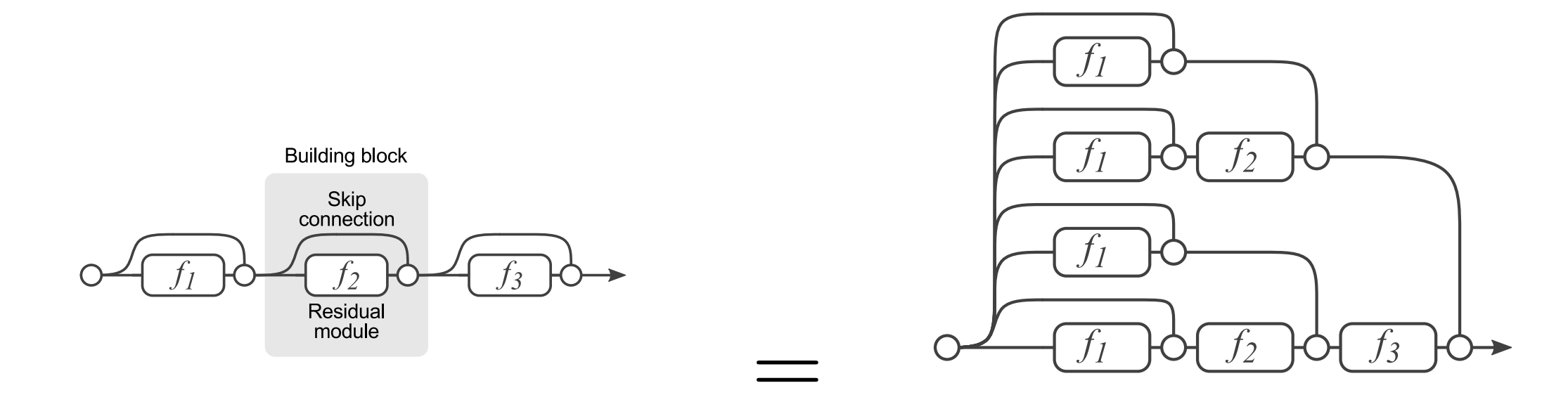
This diagram of the skip connection and its ensamble effects is from the CSGY6613 website [7]

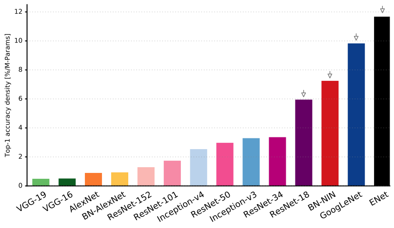Figure from Neural Network Architectures with a comparison between many of the top performaing neural network architectures by Eugenio Culurciello. You can find his full article and paper on Medium. [9]

Performance Benchmarks

From our three implementations, as well as the naive strategy that came out of the box from CORe50, we found that rehearsal is the best strategy to maintain test accuracy over different batches. The plot below shows our findings. We focus on test accuracy on task zero, in particular, because the goal of continuous learning is to remember tasks over time. It is important to point out that Rehearsal and our hybrid strategy had almost identical performance. Rehearsal and hybrid are combined because our implementations of EWC suffered dramatically, so it is safe to assume that our hybrid method performed well solely because of rehearsal.

The above line graph highlights the difficulty of continuous learning, retaining ability to predict well over time. However, the overall accuracy of the model is also very important, and our findings can be found in the figure below. It shows that the accuracy for naive and EWC do not increase throughout the batches. However, rehearsal and our hybrid method increase average accuracy throughout the batches.

Apart from test accuracy, another important metric to measure is training time. All of the code was run locally on two Macbook Pros with no more than 16 gbs of ram and no GPU usage. Because of this, training was long. Rehearsal took up to 12 hours to train. This constraint is what led us to look into less computationally and memory expensive processes, such as EWC. As you can see, EWC 02 had the fastest training time at roughly three hours. However, with our computing limited, it is recommended to use the model with this highest accuracy, because with a better computer it would run much faster.

Project Structure

The changes we made are in the following files:

• README.md: This instructions file.

• /cvpr_clvision_challenge-master/cl_ewc.py: This code is a developed using the naive_baseline.py competition file as a starting point. Running this file implement an EWC implementation 01 continual learning strategy.

• /cvpr_clvision_challenge-master/cl_rehearsal.py: This code is a developed using the naive_baseline.py competition file as a starting point. Running this file implements the rehearsal continual learning strategy.

• /cvpr_clvision_challenge-master/cl_ewc_rehearsal.py: This code is a developed using the naive_baseline.py competition file as a starting point. Running this file implements a hybrid solution using both the rehearsal continual learning strategy.

• /cvpr_clvision_challenge-master/utils/train_test.py: This code is a developed using the train_test.py naive solution competition file as a starting point. The train_net function is used for the naive and rehearsal solution strategies. The train_net_ewc has been added to train using the EWC implementation 01 strategy. The on_task_update function has been added to store the optimal weights and fisher values after training each new task.

• /cvpr_clvision_challenge-master/utils/train_test_alt_ewc.py: This file contains the second implementation of the ewc with alternative version of the both the train_net_ewc and on_task_update functions. You can see the implementation uses much less memory and time to run. In addition, using this strategy the number of fisher values and calculations does not increase with the number of tasks. However, the accuracy is not as high.

• /cvpr_clvision_challenge-master/submissions_archive/: This directory contains logs. You can find the detailed stats on successful and not so successful experimentation. In addition, there is an archive of the exact code with exact parameters used for the most successful runs.

• /cvpr_clvision_challenge-master/report_resources/: This directory images used in the readme files. See the sources for images by others in the readme text and bibliography.

• /cvpr_clvision_challenge-master/create_submission.sh: Basic bash script to run the various continual learning strategies and create the zip submission file. Simply uncomment any strategies you would like to run and comment the ones you don't want to run.

This repository is structured as follows:

• /cvpr_clvision_challenge-master/core50/: Root directory for the CORe50 benchmark, the main dataset of the challenge.
• /cvpr_clvision_challenge-master/utils/: Directory containing a few utilities methods.
• /cvpr_clvision_challenge-master/cl_ext_mem/: It will be generated after the repository setup (you need to store here eventual memory replay patterns and other data needed during training by your CL algorithm)
• /cvpr_clvision_challenge-master/submissions/: It will be generated after the repository setup. It is where the submissions directory will be created.
• /cvpr_clvision_challenge-master/fetch_data_and_setup.sh: Basic bash script to download data and other utilities.
• /cvpr_clvision_challenge-master/naive_baseline.py: Basic script to run a naive algorithm on the tree challenge categories. This script is based on PyTorch but you can use any framework you want. CORe50 utilities are framework independent.
• /cvpr_clvision_challenge-master/environment.yml: Basic conda environment to run the baselines.
• /cvpr_clvision_challenge-master/LICENSE: Standard Creative Commons Attribution 4.0 International License.

Bibliography

Research Papers/Online Resources:

1. Continuous Learning in Single-Incremental-Task Scenarios
   • This paper describes Continual Learning, Single-Incremental-Task, New Classes problem, and catastrophic forgetting. They have a great description of the Naive, Rehearsal, and Elastic Weight Consolidation approach to solving Continual Learning.
2. Overcoming catastrophic forgetting in neural networks
   • This is the first paper to propose the Elastic Weight Consolidation approach to solving Continual Learning.
3. Compete to Compute
   • This paper describes how the order of your training data matters.
4. CORe50: a New Dataset and Benchmark for Continuous Object Recognition
   • This paper describes the CORe50 dataset. In addition, the authors used the dataset to test several Continual Learning methods and compare their benchmarks.
5. Memory Efficient Experience Replay for Streaming Learning
6. Elastic Weight Consolidation (EWC): Nuts and Bolts
   • Comprehensive overview of EWC.
7. AI Spring 2020: Pantelis Course Notes
8. Stackexchange Artcle regarding ResNet18
9. Neural Network Architectures
   • Article and paper on Medimum by Eugenio Culurciello. Great comparison of top performing Neural Network Architectures.

Datasets Used:

• CORe50 Dataset
  • The dataset we use.

Code Used As a Starting Point:

• CVPR clvision challenge
  • The starting point for the code we developed. This includes the loader for the CORe50 Dataset. Also, included is the Naive approach to continual learning that we use a baseline benchmark.
• Intro To Continual Learning
  • Provided a model for the implementation of Naive, Rehearsal, and Elastic Weight Consolidation. We used this code in the development of our implementation.