The R package gdalcubes aims at making analyses of large satellite
image collections easier, faster, more intuitive, and more interactive.
The package represents the data as regular raster data cubes with
dimensions bands, time, y, and x and hides complexities in the
data due to different spatial resolutions,map projections, data formats,
and irregular temporal sampling.
- Read and process multitemporal, multispectral Earth observation image collections as regular raster data cubes by applying on-the-fly reprojection, rescaling, cropping, and resampling.
- Work with existing Earth observation imagery on local disks or cloud storage without the need to maintain a 2nd copy of the data.
- Apply user-defined R functions on data cubes.
- Execute data cube operation chains using parallel processing and lazy evaluation.
Among others, the package has been successfully used to process data from the Sentinel-2, Sentinel-5P, Landsat, PlanetScope, MODIS, and Global Precipitation Measurement Earth observation satellites / missions.
Install from CRAN with:
install.packages("gdalcubes")Installation from sources is easiest with
remotes::install_git("https://github.com/appelmar/gdalcubes")Please make sure that the git command line client is available on your system. Otherwise, the above command might not clone the gdalcubes C++ library as a submodule under src/gdalcubes.
The package builds on the external libraries GDAL, NetCDF, SQLite, and curl.
On Windows, you will need Rtools to build the package from sources.
Please install the system libraries e.g. with the package manager of your Linux distribution. Also make sure that you are using a recent version of GDAL (>2.3.0). On Ubuntu, the following commands will install all neccessary libraries.
sudo add-apt-repository ppa:ubuntugis/ppa && sudo apt-get update
sudo apt-get install libgdal-dev libnetcdf-dev libcurl4-openssl-dev libsqlite3-dev libudunits2-dev
Using Homebrew, required system libraries can be installed with
brew install pkg-config
brew install gdal
brew install netcdf
brew install libgit2
brew install udunits
brew install curl
brew install sqlite
brew install libtiff
brew install hdf5
brew install protobuf
if (!dir.exists("L8_Amazon")) {
  download.file("https://hs-bochum.sciebo.de/s/8XcKAmPfPGp2CYh/download", destfile = "L8_Amazon.zip",mode = "wb")
  unzip("L8_Amazon.zip", exdir = "L8_Amazon")
}At first, we must scan all available images once, and extract some
metadata such as their spatial extent and acquisition time. The
resulting image collection is stored on disk, and typically consumes a
few kilobytes per image. Due to the diverse structure of satellite image
products, the rules how to derive the required metadata are formalized
as collection_formats. The package comes with predefined formats for
some Sentinel, Landsat, and MODIS products (see collection_formats()
to print a list of available formats).
library(gdalcubes)

gdalcubes_options(parallel=8)

files = list.files("L8_Amazon", recursive = TRUE,
                   full.names = TRUE, pattern = ".tif")
length(files)
## [1] 1805
sum(file.size(files)) / 1024^2 # MiB## [1] 1919.12
L8.col = create_image_collection(files, format = "L8_SR", out_file = "L8.db")
L8.col
## Image collection object, referencing 180 images with 10 bands
## Images:
## name left top bottom
## 1 LC08_L1TP_226063_20140719_20170421_01_T1 -54.15776 -3.289862 -5.392073
## 2 LC08_L1TP_226063_20140820_20170420_01_T1 -54.16858 -3.289828 -5.392054
## 3 LC08_L1GT_226063_20160114_20170405_01_T2 -54.16317 -3.289845 -5.392064
## 4 LC08_L1TP_226063_20160724_20170322_01_T1 -54.16317 -3.289845 -5.392064
## 5 LC08_L1TP_226063_20170609_20170616_01_T1 -54.17399 -3.289810 -5.392044
## 6 LC08_L1TP_226063_20170711_20170726_01_T1 -54.15506 -3.289870 -5.392083
## right datetime srs
## 1 -52.10338 2014-07-19T00:00:00 EPSG:32622
## 2 -52.11418 2014-08-20T00:00:00 EPSG:32622
## 3 -52.10878 2016-01-14T00:00:00 EPSG:32622
## 4 -52.10878 2016-07-24T00:00:00 EPSG:32622
## 5 -52.11958 2017-06-09T00:00:00 EPSG:32622
## 6 -52.09798 2017-07-11T00:00:00 EPSG:32622
## [ omitted 174 images ]
##
## Bands:
## name offset scale unit nodata image_count
## 1 AEROSOL 0 1 180
## 2 B01 0 1 -9999.000000 180
## 3 B02 0 1 -9999.000000 180
## 4 B03 0 1 -9999.000000 180
## 5 B04 0 1 -9999.000000 180
## 6 B05 0 1 -9999.000000 180
## 7 B06 0 1 -9999.000000 180
## 8 B07 0 1 -9999.000000 180
## 9 PIXEL_QA 0 1 180
## 10 RADSAT_QA 0 1 180
To create a regular raster data cube from the image collection, we
define the geometry of our target cube as a data cube view, using the
cube_view() function. We define a simple overview, covering the full
spatiotemporal extent of the imagery at 1km x 1km pixel size where one
data cube cell represents a duration of one year. The provided
resampling and aggregation methods are used to spatially reproject,
crop, and rescale individual images and combine pixel values from many
images within one year respectively. The raster_cube() function
returns a proxy object, i.e., it returns immediately without doing any
expensive computations.
v.overview = cube_view(extent=L8.col, dt="P1Y", dx=1000, dy=1000, srs="EPSG:3857",
                      aggregation = "median", resampling = "bilinear")
raster_cube(L8.col, v.overview)
## A data cube proxy object
##
## Dimensions:
## low high count pixel_size chunk_size
## t 2013-01-01 2019-12-31 7 P1Y 1
## y -764014.387686915 -205014.387686915 559 1000 192
## x -6582280.06164712 -5799280.06164712 783 1000 192
##
## Bands:
## name offset scale nodata unit
## 1 AEROSOL 0 1 NaN
## 2 B01 0 1 NaN
## 3 B02 0 1 NaN
## 4 B03 0 1 NaN
## 5 B04 0 1 NaN
## 6 B05 0 1 NaN
## 7 B06 0 1 NaN
## 8 B07 0 1 NaN
## 9 PIXEL_QA 0 1 NaN
## 10 RADSAT_QA 0 1 NaN
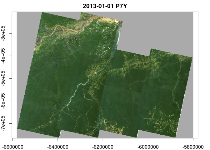
We can apply (and chain) operations on data cubes:
x = raster_cube(L8.col, v.overview) |>
  select_bands(c("B02","B03","B04")) |>
  reduce_time(c("median(B02)","median(B03)","median(B04)"))
x
## A data cube proxy object
##
## Dimensions:
## low high count pixel_size chunk_size
## t 2013-01-01 2019-12-31 1 P7Y 1
## y -764014.387686915 -205014.387686915 559 1000 192
## x -6582280.06164712 -5799280.06164712 783 1000 192
##
## Bands:
## name offset scale nodata unit
## 1 B02_median 0 1 NaN
## 2 B03_median 0 1 NaN
## 3 B04_median 0 1 NaN
plot(x, rgb=3:1, zlim=c(0,1200))library(RColorBrewer)
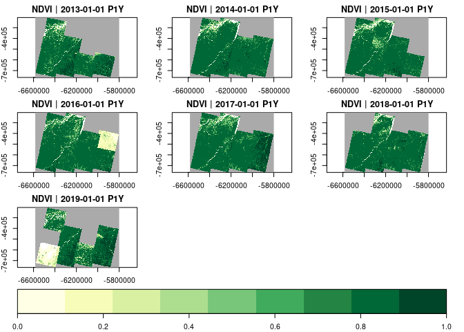
raster_cube(L8.col, v.overview) |>
select_bands(c("B04","B05")) |>
apply_pixel(c("(B05-B04)/(B05+B04)"), names="NDVI") |>
plot(zlim=c(0,1), nbreaks=10, col=brewer.pal(9, "YlGn"), key.pos=1)Calling data cube operations always returns proxy objects,
computations are started lazily when users call e.g. plot().
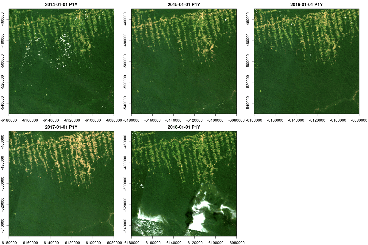
Multitemporal data cubes can be animated (thanks to the gifski package):
v.subarea.yearly = cube_view(extent=list(left=-6180000, right=-6080000, bottom=-550000, top=-450000,
                             t0="2014-01-01", t1="2018-12-31"), dt="P1Y", dx=50, dy=50,
                             srs="EPSG:3857", aggregation = "median", resampling = "bilinear")

raster_cube(L8.col, v.subarea.yearly) |>
  select_bands(c("B02","B03","B04")) |>
  animate(rgb=3:1,fps = 2, zlim=c(100,1000), width = 400,
          height = 400, save_as = "man/figures/animation.gif")
Data cubes can be exported as single netCDF files with write_ncdf(),
or as a collection of (possibly cloud-optimized) GeoTIFF files with
write_tif(), where each time slice of the cube yields one GeoTIFF
file. Data cubes can also be converted to terra or starsobjects:
raster_cube(L8.col, v.overview) |>
  select_bands(c("B04","B05")) |>
  apply_pixel(c("(B05-B04)/(B05+B04)"), names="NDVI") |>
  write_tif() |>
  terra::rast() -> x
x
## class : SpatRaster
## dimensions : 559, 783, 7 (nrow, ncol, nlyr)
## resolution : 1000, 1000 (x, y)
## extent : -6582280, -5799280, -764014.4, -205014.4 (xmin, xmax, ymin, ymax)
## coord. ref. : WGS 84 / Pseudo-Mercator (EPSG:3857)
## sources : cube_845e62ea0e0a2013-01-01.tif
## cube_845e62ea0e0a2014-01-01.tif
## cube_845e62ea0e0a2015-01-01.tif
## ... and 4 more source(s)
## names : NDVI, NDVI, NDVI, NDVI, NDVI, NDVI, ...
raster_cube(L8.col, v.overview) |>
  select_bands(c("B04","B05")) |>
  apply_pixel(c("(B05-B04)/(B05+B04)"), names="NDVI") |>
  stars::st_as_stars() -> y
y
## stars object with 3 dimensions and 1 attribute
## attribute(s), summary of first 1e+05 cells:
## Min. 1st Qu. Median Mean 3rd Qu. Max. NA's
## NDVI -0.5595199 0.4207425 0.723503 0.5765454 0.849606 0.8892204 79500
## dimension(s):
## from to offset delta refsys point
## x 1 783 -6582280 1000 WGS 84 / Pseudo-Mercator NA
## y 1 559 -205014 -1000 WGS 84 / Pseudo-Mercator NA
## time 1 7 NA NA POSIXct FALSE
## values x/y
## x NULL [x]
## y NULL [y]
## time [2013-01-01,2014-01-01),...,[2019-01-01,2020-01-01)
To reduce the size of exported data cubes, compression and packing (conversion of doubles to smaller integer types) are supported.
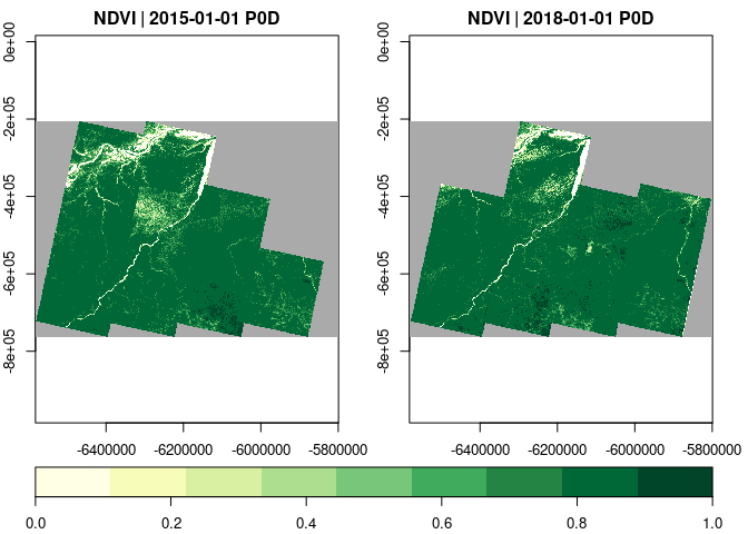
If only specific time slices of a data cube are needed, select_time()
can be called before plotting / exporting.
raster_cube(L8.col, v.overview) |>
  select_bands(c("B04","B05")) |>
  apply_pixel(c("(B05-B04)/(B05+B04)"), names="NDVI") |>
  select_time(c("2015", "2018")) |>
plot(zlim=c(0,1), nbreaks=10, col=brewer.pal(9, "YlGn"), key.pos=1)Users can pass custom R functions to reduce_time() and
apply_pixel(). Below, we derive a greenest pixel composite by
returning RGB values from pixels with maximum NDVI for all pixel
time-series.
v.subarea.monthly = cube_view(view = v.subarea.yearly, dt="P1M", dx = 100, dy = 100,
                              extent = list(t0="2015-01", t1="2018-12"))
raster_cube(L8.col, v.subarea.monthly) |>
  select_bands(c("B02","B03","B04","B05")) |>
  apply_pixel(c("(B05-B04)/(B05+B04)"), names="NDVI", keep_bands=TRUE) |>
  reduce_time(names=c("B02","B03","B04"), FUN=function(x) {
    if (all(is.na(x["NDVI",]))) return(rep(NA,3))
    return (x[c("B02","B03","B04"), which.max(x["NDVI",])])
  }) |>
plot(rgb=3:1, zlim=c(100,1000))In many cases, one is interested in extracting sets of points, time
series, or summary statistics over polygons, e.g., to generate training
data for machine learning models. Package version 0.6 therefore
introduces the extract_geom() function, which replaces the previous
implementations in query_points(), query_timeseries(), and
zonal_statistics().
Below, we randomly select 100 locations and query values of single data cube cells and complete time series.
x = runif(100, v.overview$space$left, v.overview$space$right)
y = runif(100, v.overview$space$bottom, v.overview$space$top)
t = sample(as.character(2013:2019), 100, replace = TRUE)
df = sf::st_as_sf(data.frame(x = x, y = y), coords = c("x", "y"), crs = v.overview$space$srs)

# spatiotemporal points
raster_cube(L8.col, v.overview) |>
  select_bands(c("B04","B05")) |>
  extract_geom(df, datetime = t) |>
  dplyr::sample_n(15) # print 15 random rows
## FID time B04 B05
## 21 95 2016-01-01 182.3935 3360.3492
## 50 11 2016-01-01 282.0869 3039.4177
## 34 96 2018-01-01 885.3366 3565.0468
## 54 4 2019-01-01 171.4910 2825.5037
## 38 1 2018-01-01 249.7769 3091.6986
## 42 64 2018-01-01 315.9540 3326.0070
## 3 18 2014-01-01 720.9067 3689.0444
## 55 47 2019-01-01 569.0251 2844.1652
## 22 74 2017-01-01 264.0236 3036.4862
## 29 73 2017-01-01 198.0629 3135.8718
## 39 38 2018-01-01 201.2096 2882.1543
## 28 30 2017-01-01 171.2704 2754.2129
## 61 27 2019-01-01 405.6078 588.0934
## 51 25 2019-01-01 150.7253 2886.3868
## 25 19 2016-01-01 3593.0970 5285.5944
# time series at spatial points
raster_cube(L8.col, v.overview) |>
  select_bands(c("B04","B05")) |>
  extract_geom(df) |>
  dplyr::sample_n(15) # print 15 random rows
## FID time B04 B05
## 319 98 2017-01-01 217.7226 3296.470
## 25 86 2013-01-01 199.9388 2844.481
## 100 58 2014-01-01 202.8860 2869.232
## 256 43 2017-01-01 280.8320 3187.573
## 390 41 2019-01-01 149.7427 2879.540
## 60 45 2013-01-01 239.1001 3219.560
## 288 85 2016-01-01 309.2750 2876.053
## 290 24 2017-01-01 238.6707 3151.653
## 135 31 2015-01-01 951.8869 3004.181
## 315 4 2017-01-01 146.7365 2891.950
## 66 18 2015-01-01 436.6083 3535.842
## 381 96 2019-01-01 190.6946 2812.518
## 40 49 2013-01-01 169.4907 2761.769
## 284 33 2016-01-01 225.0206 2925.426
## 222 45 2016-01-01 295.2418 3153.687
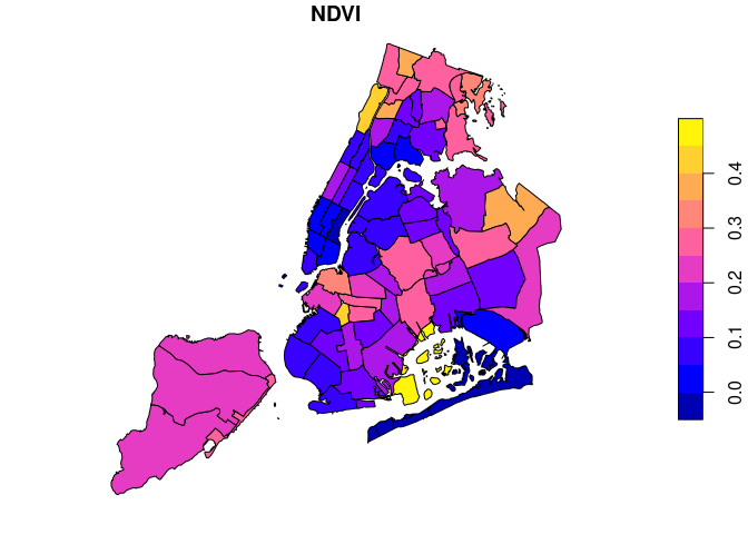
In the following, we use the example Landsat dataset (reduced resolution) from the package and compute median NDVI values within some administrative regions in New York City. The result is a data.frame containing data cube bands, feature IDs, and time as columns.
L8_files <- list.files(system.file("L8NY18", package = "gdalcubes"),
                       ".TIF", recursive = TRUE, full.names = TRUE)
v = cube_view(srs="EPSG:32618", dy=300, dx=300, dt="P1M",
              aggregation = "median", resampling = "bilinear",
              extent=list(left=388941.2, right=766552.4,
                          bottom=4345299, top=4744931,
                          t0="2018-01", t1="2018-12"))
sf = sf::st_read(system.file("nycd.gpkg", package = "gdalcubes"), quiet = TRUE)

raster_cube(create_image_collection(L8_files, "L8_L1TP"), v) |>
  select_bands(c("B04", "B05")) |>
  apply_pixel("(B05-B04)/(B05+B04)", "NDVI") |>
  extract_geom(sf, FUN = median) -> zstats

dplyr::sample_n(zstats, 15) # print 15 random rows
## FID time NDVI
## 1 68 2018-03-01 0.008483257
## 2 49 2018-05-01 0.041807600
## 3 41 2018-01-01 -0.012513485
## 4 47 2018-10-01 0.002116781
## 5 71 2018-08-01 0.255297575
## 6 26 2018-12-01 0.060638615
## 7 48 2018-06-01 0.055183957
## 8 56 2018-10-01 0.138487053
## 9 25 2018-10-01 0.093297342
## 10 58 2018-04-01 0.022237839
## 11 57 2018-12-01 0.053809129
## 12 43 2018-08-01 0.065916489
## 13 2 2018-08-01 0.130797459
## 14 31 2018-10-01 0.044141370
## 15 32 2018-01-01 0.058137169
We can combine the result with the original features by a table join on
the FID column using merge():
sf$FID = rownames(sf)
x = merge(sf, zstats, by = "FID")
plot(x[x$time == "2018-07-01", "NDVI"])
When using input features with additional attributes / labels, the
extract_geom() function hence makes it easy to create training data
for machine learning models.
Cloud support with STAC: gdalcubes can be used directly on cloud
computing platforms including Amazon Web Services, Google Cloud
Platform, and Microsoft Azure. Imagery can be read from their open data
catalogs and discovered by connecting to STAC API endpoints using the
rstac package (see links
at the end of this page).
Machine learning: The built-in functions extract_geom and
predict help to create training data and apply predictions on data
cubes using machine learning models as created from packages caret or
tidymodels.
Further operations: The previous examples covered only a limited set
of built-in functions. Further data cube operations for example include
spatial and/or temporal slicing (slice_time, slice_space), cropping
(crop), application of moving window / focal operations
(window_time, window_space), filtering by arithmetic expressions on
pixel values and spatial geometries (filter_pixel, filter_geom), and
combining two or more data cubes with identical shape (join_bands).
- Official R package website
- Tutorial on YouTube how to use gdalcubes in the cloud, streamed at OpenGeoHub Summer School 2021
- 1st blog post on r-spatial.org
- 2nd blog post on r-spatial.org describing how to use gdalcubes in cloud-computing environments
- Open access paper in the special issue on Earth observation data cubes of the data journal
