The main goal of this project is to design, create and build pipeline that detects and tracks vehicles in a given video from a camera mounted in the front of a car.
In order to achieve this goal, some computer vision and machine learning techniques were applied. The first important stage was to define and extract the relevant features from the images applying gradients and transformations to them.
Once the features were properly extracted a Linear SVM classifier was trained with the GTI vehicle image database and the KITTI vision benchmark suite datasets.
Finally, applying a sliding-window technique, we searched for vehicles in the images, pointed them with a surrounding rectangle.
The steps of this project are the following:
- Perform a Histogram of Oriented Gradients (HOG) feature extraction on a labeled training set of images and train a Linear SVM classifier
- Optionally, you can also apply a color transformation and append binned color features, as well as histograms of color, to your HOG feature vector.
- Note: for those first two steps don't forget to normalize your features and randomize a selection for training and testing.
- Implement a sliding-window technique and use your trained classifier to search for vehicles in images.
- Run your pipeline on a video stream (start with the test_video.mp4 and later implement on full project_video.mp4) and create a heat map of recurring detections frame by frame to reject outliers and follow detected vehicles.
- Estimate a bounding box for the detected vehicles
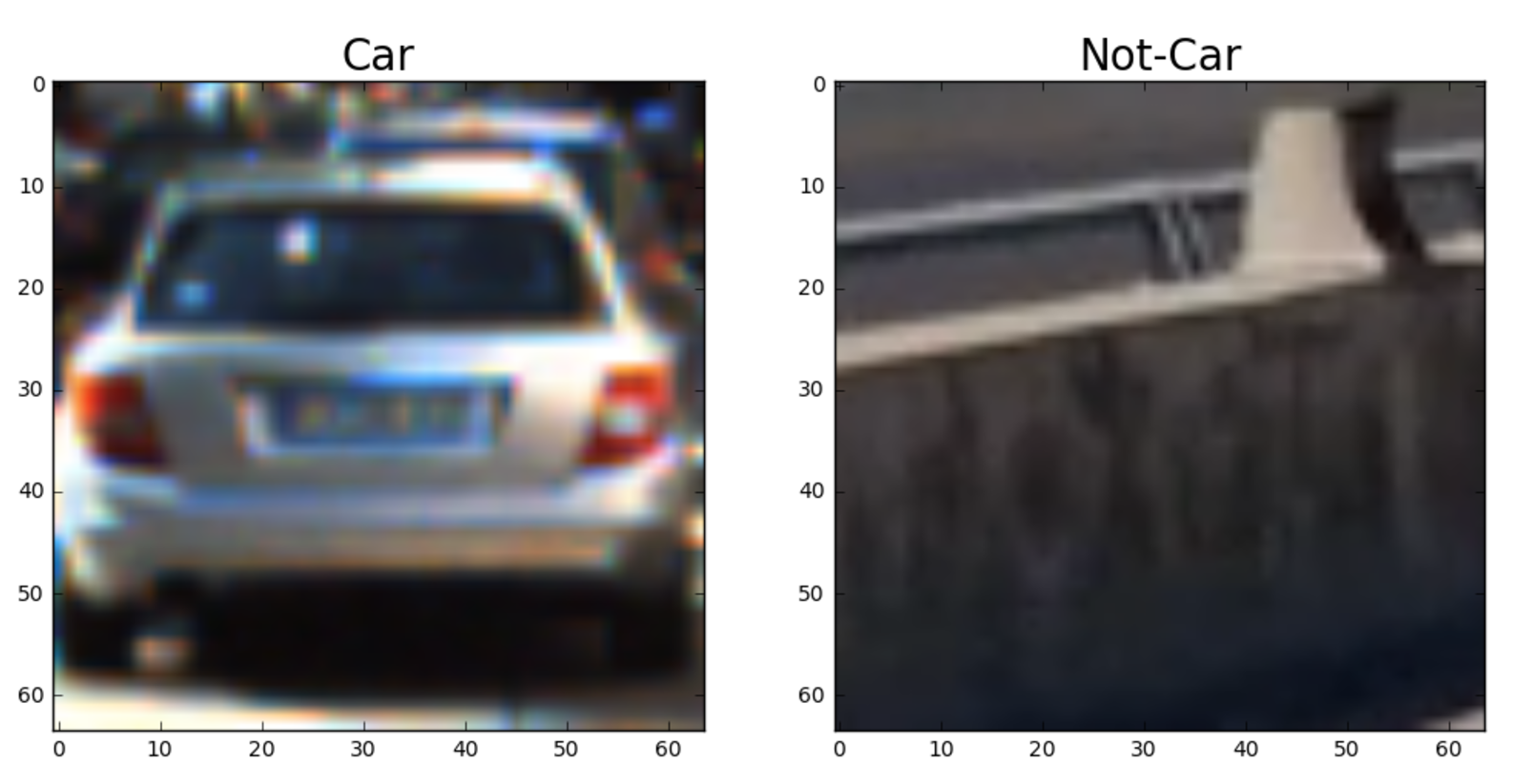
First, we needed to explore the datasets to understand the problem we wanted to solve. Both datasets contain a bunch of examples of car and not-car images. The images are in color and have a size of 64 by 64 pixels. Besides, they can only belong to one of these classes. The labels are given by the name of the folder where the images are stored.
As it was mentioned before, we wanted to extract the relevant features from the images in order to be able to detect vehicles. Because the HOG technique works very well in these scenarios, it was decided to apply it to the images.
Said that, the key point here was not to decide if apply HOG or not but how to apply it instead, or in other words to select a set of proper values.
It is also important to mention that the parameters not only have an effect in terms of detection but also in terms of performance. It is not the same to select 9 than 11 orientations. As well as it is not the same either, to select 32 pixels_per_cell than 8. The chosen parameters are explained in the following section.
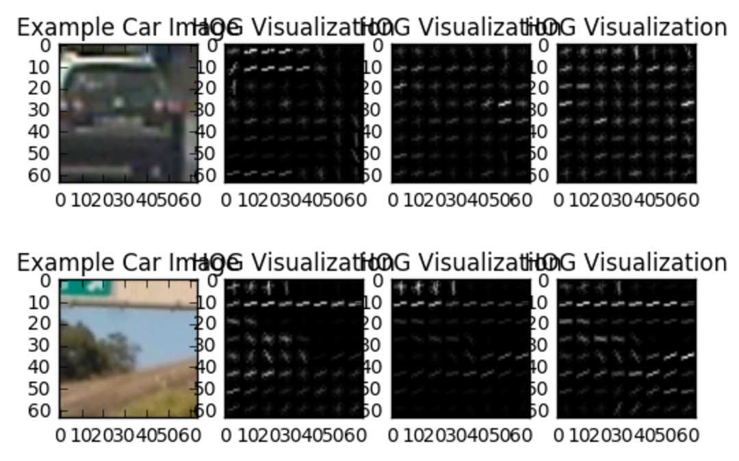
To introduce some results, in the following image it can be seen an example using the YCrCb color space and HOG parameters of orientations=9, pixels_per_cell=(8, 8) and cells_per_block=(2, 2):
cspace = 'YCrCb' # Can be RGB, HSV, LUV, HLS, YUV, YCrCb
orient = 9
pix_per_cell = 8
cell_per_block = 2
hog_channel = "ALL" # Can be 0, 1, 2, or "ALL"

# Check the HOG extraction

cars = glob.glob('./data/vehicles/*/*.png')
notcars = glob.glob('./data/non-vehicles/*/*.png')

random_index = np.random.randint(0, len(cars))

img = cars[random_index]
features, hog_image = features_for_vis(mpimg.imread(img), cspace=cspace,
                        pix_per_cell=pix_per_cell, cell_per_block=cell_per_block,
                        hog_channel=hog_channel)

fig = plt.figure()
plt.subplot(1, len(hog_image)+1, 1)
plt.imshow(mpimg.imread(img))
plt.title('Example Car Image')
for idx, hog_img in enumerate(hog_image):
  plt.subplot(1, len(hog_image)+1, idx+2)
  plt.imshow(hog_img, cmap='gray')
plt.title('HOG Visualization')In the first approach, some helper functions were defined to visualize the HOG features from the images. After that, some functions were redefined and the final values for the parameters were the following:
cspace = 'YCrCb' # Can be RGB, HSV, LUV, HLS, YUV, YCrCb
orient = 9  # HOG orientations
pix_per_cell = 8 # HOG pixels per cell
cell_per_block = 2 # HOG cells per block
hog_channel = "ALL" # Can be 0, 1, 2, or "ALL"
spatial_size = (32, 32) # Spatial binning dimensions
hist_bins = 32    # Number of histogram bins
spatial_feat = True # Spatial features on or off
hist_feat = True # Histogram features on or off
hog_feat = True # HOG features on or off
At the beginning we tried with HLS and HSV color spaces but after several trial and error phases it seemed that YUV and YCrCb performed better. Finally, the YCrCb was selected with a number of 9 HOG orientations. It could be said that is a balanced number between extracting enough number of features but no so many because it could slow down the training phase.
Instead of selecting just one channel, we processed all channels of the images. The spatial and color extraction were also taken into account to build the final features.
The final feature vector length was of 8096 in total.
When the feature vectors were built, we set some other important steps before the training phase.
- Fit a per-scaler and normalize the features from the transformations and HOG extraction
- Split up data into randomized training and test sets thanks to the
train_test_split()method
The final model was based on a Linear SVM Classifier. The training phase was successfully passed with a 99.25% of accuracy in the test set in less than 60 seconds. The SVM performs very well in image classification issues so we didn't need to try other different models.
As it can be seen, we stay with the default parameters of the SVM (gamma or C)
# Use a linear SVC
svc = LinearSVC()
# Check the training time for the SVC
t=time.time()
svc.fit(X_train, y_train)
t2 = time.time()
print(round(t2-t, 2), 'Seconds to train SVC...')
# Check the score of the SVC
print('Test Accuracy of SVC = ', round(svc.score(X_test, y_test), 4))
# Check the prediction time for a single sample
t=time.time()
n_predict = 10
print('My SVC predicts: ', svc.predict(X_test[0:n_predict]))
print('For these',n_predict, 'labels: ', y_test[0:n_predict])
t2 = time.time()
print(round(t2-t, 5), 'Seconds to predict', n_predict,'labels with SVC')
Once the model was properly trained, the resulting values were stored in a .pkl file to avoid repeating the same steps and continue with the following steps from here.
The solution was based on 64 by 64 images of vehicles and not-vehicles. And at the same time, the goal of this project was to detect vehicles in a video mounted in the front of a car. In order to fit the current input in our model it was necessary to apply a sliding window search along the images to extract pieces from them and convert them in something that the model can processes.
To achieve that goal, it was necessary to apply a sliding window search technique, where basically the image is divided into N pieces, and each one is separately processed.
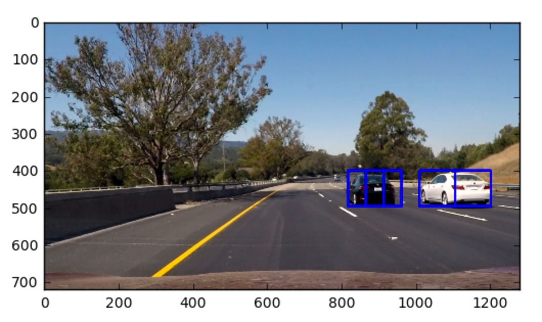
Looking at the following code, the slide_window() method defines the grid of the windows and then, the search_windows() method searches (resizes, extracts and scales the features, and predicts using the model) for a vehicle in each one.
windows = slide_window(image, x_start_stop=[None, None], y_start_stop=y_start_stop,
                    xy_window=(96, 96), xy_overlap=(0.5, 0.5))

hot_windows = search_windows(image, windows, svc, X_scaler, color_space=cspace,
                        spatial_size=spatial_size, hist_bins=hist_bins,
                        orient=orient, pix_per_cell=pix_per_cell,
                        cell_per_block=cell_per_block,
                        hog_channel=hog_channel, spatial_feat=spatial_feat,
                        hist_feat=hist_feat, hog_feat=hog_feat)

window_img = draw_boxes(draw_image, hot_windows, color=(0, 0, 255), thick=6)
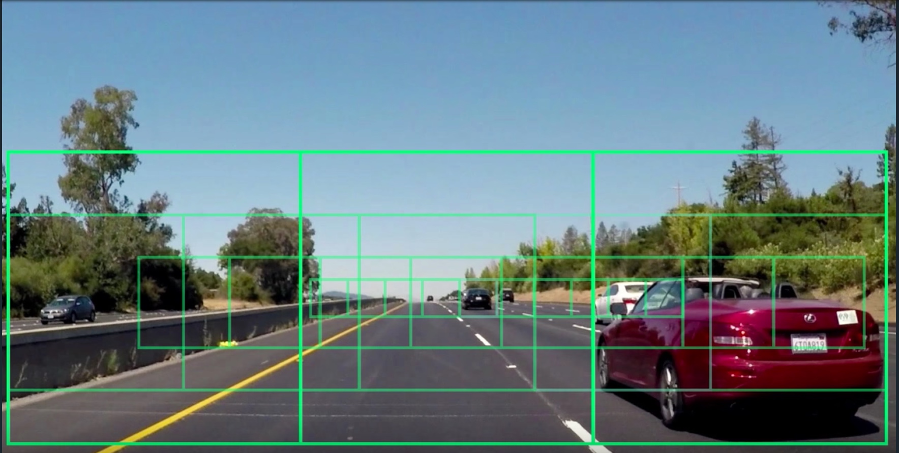
After that and once we checked the model was working fine, it was defined a smarter windows definition. Instead of just defining a fixed-size window, some different windows layers were defined. We did that to approximate the window parameters to the kind of elements that we wanted to find in the images.
window_configs = [
  {
    "x_start_stop": [None, None],
    "y_start_stop": [400, 656],
    "xy_window": (256, 256),
    "xy_overlap": (0.5, 0.5)
  },
  {
    "x_start_stop": [None, None],
    "y_start_stop": [400, 656],
    "xy_window": (128, 128),
    "xy_overlap": (0.6, 0.5)
  },
  {
    "x_start_stop": [100, 1280],
    "y_start_stop": [400, 500],
    "xy_window": (96, 96),
    "xy_overlap": (0.7, 0.5)
  },
  {
    "x_start_stop": [500, 1280],
    "y_start_stop": [400, 500],
    "xy_window": (48, 48),
    "xy_overlap": (0.7, 0.5)
  }
]
Large windows of 256 by 256 from pixel 400 to pixel 656 in the Y coordinate. Medium windows of 128 by 128 from pixel 400 to pixel 656 in the Y coordinate. Small windows of 96 by 96 from pixel 400 to pixel 500 in the Y coordinate. The X range was restricted to stop the process performance being worse. X-Small windows of 48 by 48 from pixel 400 to pixel 500 in the Y coordinate. The X range was also restricted in this case.
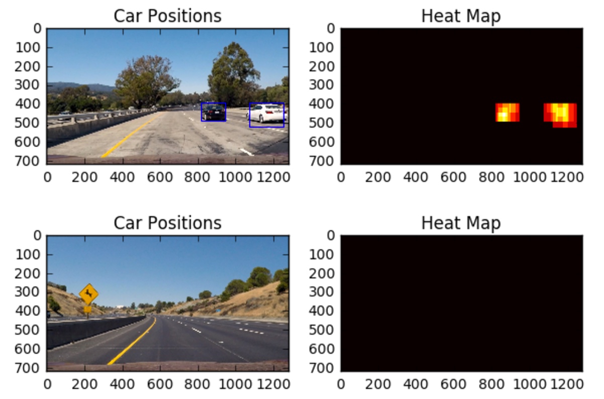
At the end of this process, we had several matched boxes where vehicles should hopefully appear. Taking all windows, we also created heatmaps generating new arrays with ones in the pixels where a vehicle was detected. Having these heatmaps and applying the scipy.ndimage.measurements.label() method we were able to define the final rectangles from all matching boxes.
At this point, the majority of the pipeline has been already explained. Doing some recap, we got a trained Linear SVM classifier with vehicles and not-vehicles data and a pipeline that split a given image in windows and then try to know if there is or not a vehicle in each window.
After applying different window-layers (different positions, sizes and overlap), we built a heatmap of points where a vehicle was detected.
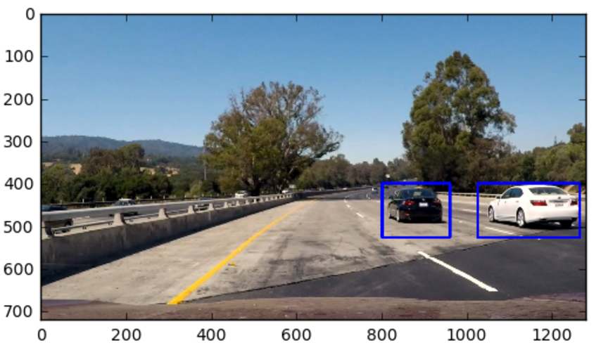
Once we knew the whole area where a vehicle could be likely found, it was required to point that area with a rectangle. In other scenario this could be an input for a hypothetical driving car agent.
Finally, to generate the video, it was applied the same pipeline that as to the images. In this case it was also defined a simplified python class to have control of the frame number and the last calculated boxes.
class Video(object):

  def __init__(self):
    self.frame_count = 0
    self.last_labels = None

  def update(self):
    self.frame_count += 1
Instead of calculating the boxes in each frame, it was applied a filter in order to reduce the processing time. Moreover it was useless to estimate them each 1/30 seconds.
At this point and with the current algorithm we were able to detect the vehicles in the images but it was also possible to detect some sudden "ghost cars" (false positives) in parts of not-cars in the image. Because we were filtering, it was weird to have a continuous false positives in a particular position of the image. Instead of that, sometimes it could appear some flickering, from a bad prediction of the model. To avoid this non-desired behavior, it was set a threshold algorithm where at least 2 or 3 boxes have to overlay each other in order to consider it a real vehicle detection.
heat = add_heat(heat,all_windows) # all_windows (detected windows)
heat = apply_threshold(heat,3)
labels = label(heat)
video.last_labels = labels
draw_image = draw_labeled_bboxes(draw_image, labels)
return draw_image
Here's a link to THE YOUTUBE VIDEO
After testing the pipeline several times, it could be said that the model works fine in standard conditions. In general, the key point was related to choose a good set of parameters for the feature extraction. The SVM model performed well in any case but the images processing was really important.
The quality of the video is quite good so that the model predicts correctly the majority of the time. Probably in other scenarios with worse weather or light conditions, the model wouldn't be able to detect vehicles in the same way as it does.
In a real-world environment more advanced techniques should be applied but at the end the concepts of extracting features applying transformations and HOG should be also present. We could also say that in order to create a more robust system it would be necessary to have a larger and more complex datasets with different vehicle models, roads, light and weather conditions, etc.
However it's really impressive how designing a computer-vision-techniques based pipeline and training a "not-too-complicated" classification model, we were able to build a complete system that detects real cars in real videos from a camera.
Some ways to improve the current model could be:
- Configure more advanced windows-layers.
- Design and train more sophisticated models.
- Think about a more advanced vehicle tracking algorithm once a vehicle has been properly detected and avoid blind searching on each frame.
- Set smarter thresholds to avoid detecting false positives.

