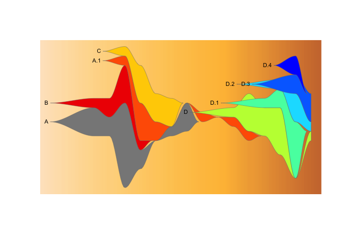
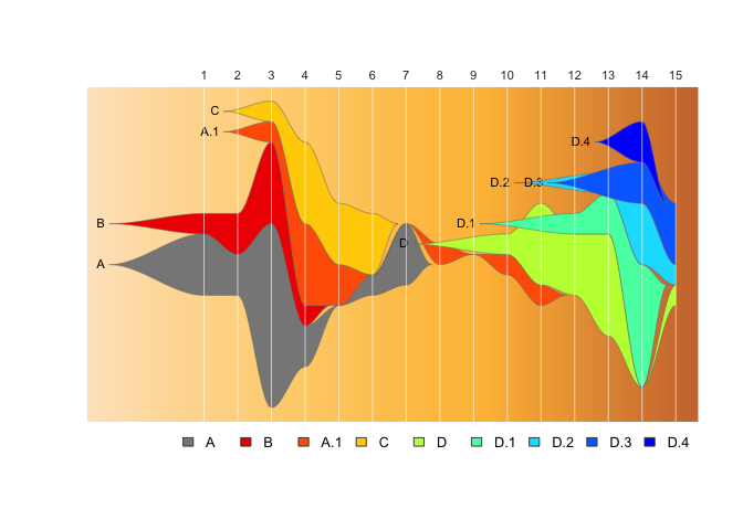
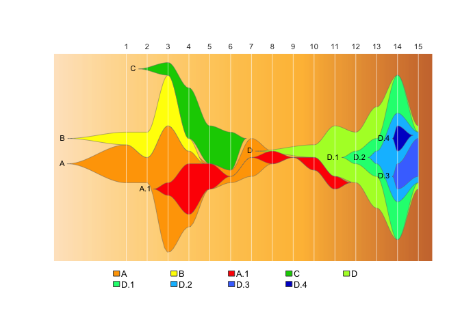
This package provides tools to use Chris Miller’s fishplot package (https://github.com/chrisamiller/fishplot) with epidemiological datasets, to generate fishplot epi-curves.
Why?
A fishplot is variety of themeriver / streamgraph, which is designed specifically for categorical data where where individual categories can mutate to form subcategories. Originally designed for plotting evolution of tumor cell lineages, we have found fishplots especially useful for illustrating the rise and fall of genomic clusters in disease outbreaks, which can have a similar evolutionary pattern.
However, a count matrix for a fishplot has a set of specific rules which an epidemiological dataset will not naturally fulfill:
- cluster counts per timepoint can never go completely to zero, if cases reappear later
- if a cluster has a parent/child relationship, at every timepoint the parent must always have >= the count of all its children.
- counts should be normalised to fit the fishplot y-axis
This package exists to make it easy to convert a list of samples in an
epidemological dataset into a normalised and appropriately “padded”
relative count matrix that fulfils these requirements.
- Installation
- Usage
- Input/Output
- Calculate timepoints
- Using informative timepoint labels
- Controlling appearance
- Citation
- Acknowledgements
You can install epifish with:
#install devtools if you don't have it already
install.packages("devtools")
library(devtools)

#install epifish
devtools::install_github("learithe/epifish")To get started with a basic epi fishplot, given an input file in the right format (details below), this is all you need:
# load required libraries
library(fishplot); library(epifish)
#> Using fishPlot version 0.5.1

# read data file
sample_df <- read.csv(system.file("extdata/samples.csv", package = "epifish"), stringsAsFactors=FALSE)

# run epifish
epifish_output <- build_epifish( sample_df )
#> Checking for missing timepoints:
#>  - Adding zero counts for missing timepoint: 9
#> The maximum sample count per timepoint (height of Y-axis) is:  15

# run fishplot on the epifish output
fishplot::fishPlot( epifish_output$fish, shape="spline" )
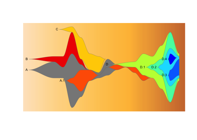
If you want to include evolutionary relationships with subclusters:
# load required libraries
library(fishplot); library(epifish)

# read data files
sample_df <- read.csv(system.file("extdata/samples.csv", package = "epifish"), stringsAsFactors=FALSE)
parent_df <- read.csv(system.file("extdata/parents.csv", package = "epifish"), stringsAsFactors=FALSE)

# run epifish
epifish_output <- build_epifish( sample_df, parent_df )
#> Checking for missing timepoints:
#>  - Adding zero counts for missing timepoint: 9
#> setting parent position of child A.1  to  1
#> setting parent position of child D.3  to  7
#> setting parent position of child D.2  to  6
#> setting parent position of child D.1  to  5
#> setting parent position of child D.4  to  7
#> Padding parent values in matrix:
#> adding child  D.4  to parent  D.2
#> adding child  D.3  to parent  D.2
#> adding child  D.2  to parent  D.1
#> adding child  D.1  to parent  D
#> adding child  A.1  to parent  A
#> The maximum sample count per timepoint (height of Y-axis) is:  15

# run fishplot on the epifish output
fishPlot( epifish_output$fish, shape="spline" ) This demo expands on the quick-start example. It runs on a made-up set
of example data that can be accessed here, in the
inst/extdata directory.
Load epifish and required packages
library(fishplot); library(epifish)Read in the tables of sample data, cluster parent-child relationships, and custom colour scheme:
sample_df <- read.csv(system.file("extdata/samples.csv", package = "epifish"), stringsAsFactors=FALSE)
parent_df <- read.csv(system.file("extdata/parents.csv", package = "epifish"), stringsAsFactors=FALSE)
colour_df <- read.csv(system.file("extdata/colours.csv", package = "epifish"), stringsAsFactors=FALSE)
Use epifish to convert this into a fishplot object, with extra assorted summary information:
epifish_output <- build_epifish( sample_df, parent_df=parent_df, colour_df=colour_df, add_missing_timepoints=TRUE)
#> Checking for missing timepoints:
#>  - Adding zero counts for missing timepoint: 9
#> setting parent position of child A.1  to  1
#> setting parent position of child D.3  to  7
#> setting parent position of child D.2  to  6
#> setting parent position of child D.1  to  5
#> setting parent position of child D.4  to  7
#> Padding parent values in matrix:
#> adding child  D.4  to parent  D.2
#> adding child  D.3  to parent  D.2
#> adding child  D.2  to parent  D.1
#> adding child  D.1  to parent  D
#> adding child  A.1  to parent  A
#> The maximum sample count per timepoint (height of Y-axis) is:  15
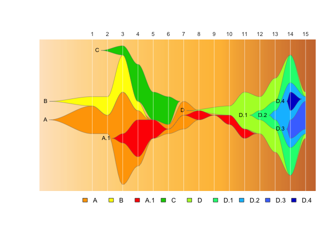
Then use the fishplot package to generate a fishplot:
fishPlot(epifish_output$fish, shape="spline",
         vlines=epifish_output$timepoints, vlab=epifish_output$timepoints)
drawLegend(epifish_output$fish, nrow=1)
If you’re happy with the default colours, or all your clusters are independent, you don’t need those dataframes:
epifish_output <- build_epifish( sample_df )
#> Checking for missing timepoints:
#>  - Adding zero counts for missing timepoint: 9
#> The maximum sample count per timepoint (height of Y-axis) is:  15

fishPlot(epifish_output$fish, shape="spline",
         vlines=epifish_output$timepoints, vlab=epifish_output$timepoints)
drawLegend(epifish_output$fish, nrow=1)
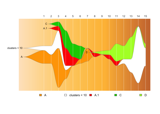
You also can automatically collapse any clusters of a minimum size into
a group with min_cluster_size:
Note: this currently does not work well with parent/child relationships
if any child clusters are small!
epifish_output <- build_epifish(sample_df, colour_df=colour_df, min_cluster_size=10)
#> Checking for missing timepoints:
#>  - Adding zero counts for missing timepoint: 9
#> Warning in set_fish_colours(colour_df, fishplot_names):
#> WARNING: existing clusters not found in colour list, setting these to white: clusters < 10
#> Warning in set_fish_colours(colour_df, fishplot_names):
#> WARNING: some clusters in colour list not found in data: B, D.1, D.2, D.3, D.4
#> The maximum sample count per timepoint (height of Y-axis) is:  15

fishPlot(epifish_output$fish, shape="spline", vlines=epifish_output$timepoints, vlab=epifish_output$timepoints)
drawLegend(epifish_output$fish, nrow=1)Example input files/templates can be found in the inst/extdata folder
or with system.file(..., package = "epifish"). The basic requirement
is a data frame containing one row per sample, with columns cluster_id
and timepoint (any other columns are ignored). Optionally, the
timepoint column can be calculated using epifish from a column of
dates (see below).
Optional data frames may also be provided that describe parent-child relationships for clusters (eg cluster A.1 evolved from cluster A), or a custom colour scheme.
It is easiest and safest (especially when working with dates) to save
and maintain these tables in .csv (comma-separated values) format, and
to read them into R using read.csv("filename", stringsAsFactors=FALSE)
as shown in the example above. However you can use whatever methods you
want to create these dataframes, as long as they contain the required
columns in character or numeric (NOT factor) format.
the last few rows of sample data:
(Note that the order doesn’t matter)
| case_id | cluster_id | date_of_collection | timepoint |
|---|---|---|---|
| 80 | D.3 | 9/4/2020 | 15 |
| 81 | D.4 | 2/4/2020 | 14 |
| 82 | D.4 | 2/4/2020 | 14 |
| 83 | D.3 | 3/4/2020 | 14 |
| 85 | D.3 | 3/4/2020 | 14 |
| 84 | A.1 | 22/1/2020 | 4 |
the parent-child data:
| cluster | parent |
|---|---|
| A | |
| A.1 | A |
| B | |
| C | |
| D | |
| D.3 | D.2 |
| D.2 | D.1 |
| D.1 | D |
| D.4 | D.2 |
a custom colour scheme:
(Note that you can use named ggplot
colours
or hex codes (eg “red” or “#ff0000”) )
| cluster | colour |
|---|---|
| A | orange |
| A.1 | red |
| B | yellow |
| C | green3 |
| D | greenyellow |
| D.1 | springgreen |
| D.2 | deepskyblue |
| D.3 | royalblue1 |
| D.4 | blue3 |
The output of epifish is a list variable (named epifish_output here)
containing: a fishplot object (epifish_output$fish), the data
structures needed to generate it, and some extra data summary tables:
fishfishplot object to pass tofishplot::fishPlot()timepoint_countssummary table of number of samples per cluster per timepointtimepoint_sumssummary table of number of samples per timepointcluster_sumssummary table of total number of samples per clustertimepointsvector of timepoints usedtimepoint_labelsvector of the names of timepoints assigned in the plotparentsnamed list matching child clusters to their parent’s position in the matrix (0 means cluster is independent)raw_tableinitial table of counts per cluster per timepoint, before padding and normalisationfish_tablenormalised and parent-padded table for the epi-fishplotfish_matrixfinal transformed matrix used to make the epifish object
The epifish fishplot object output epifish_output$fish is used with
the fishplot package’s fishPlot() function to generate an R plot
image, as shown above. If using RStudio, it is most straightforward to
save the R plot as PDF image from the RStudio plot window (Export ->
“Save as PDF”).
If you wish to save individual tables from the epifish output list for any reason, it can be done like so:
write.csv(epifish_output$fish_table, "epifishplot_table.csv", row.names=FALSE)This is the extra summary data that epifish creates:
# total cases per cluster per timepoint
print( as.data.frame(epifish_output$timepoint_counts), row.names=FALSE )
#>  timepoint FPCluster n
#>          1         A 3
#>          1         B 1
#>          2         A 2
#>          2         B 2
#>          3         A 9
#>          3       A.1 1
#>          3         B 4
#>          3         C 1
#>          4         A 2
#>          4       A.1 4
#>          4         B 1
#>          4         C 4
#>          5       A.1 2
#>          5         C 3
#>          6         A 1
#>          6         C 3
#>          7         A 3
#>          8       A.1 1
#>          9         A 0
#>          9         B 0
#>          9       A.1 0
#>          9         C 0
#>          9         D 0
#>          9       D.1 0
#>          9       D.2 0
#>          9       D.3 0
#>          9       D.4 0
#>         10       A.1 1
#>         10         D 1
#>         11       A.1 1
#>         11         D 4
#>         12         D 3
#>         12       D.1 1
#>         13         D 5
#>         13       D.1 2
#>         13       D.2 1
#>         14       D.1 6
#>         14       D.2 3
#>         14       D.3 2
#>         14       D.4 2
#>         15         D 1
#>         15       D.2 1
#>         15       D.3 3

# total cases per timepoint
print( as.data.frame(epifish_output$timepoint_sums), row.names=FALSE )
#>  timepoint  n
#>          1  4
#>          2  4
#>          3 15
#>          4 11
#>          5  5
#>          6  4
#>          7  3
#>          8  1
#>          9  0
#>         10  2
#>         11  5
#>         12  4
#>         13  8
#>         14 13
#>         15  5

# total cases per cluster
print( as.data.frame(epifish_output$cluster_sums), row.names=FALSE )
#>  FPCluster n
#>          A 7
#>        A.1 7
#>          B 5
#>          C 5
#>          D 6
#>        D.1 4
#>        D.2 4
#>        D.3 3
#>        D.4 2

# parent relationship table
print( epifish_output$parents )
#>   A   B A.1   C   D D.1 D.2 D.3 D.4
#>   0   0   1   0   0   5   6   7   7

# list of timepoints to display
print( epifish_output$timepoints )
#>  1  2  3  4  5  6  7  8  9 10 11 12 13 14 15
#>  1  2  3  4  5  6  7  8  9 10 11 12 13 14 15

# list of labels for each timepoint
print( epifish_output$timepoint_labels )
#>  [1] "1"  "2"  "3"  "4"  "5"  "6"  "7"  "8"  "9"  "10" "11" "12" "13" "14" "15"

# raw count table
print( epifish_output$raw_table )
#>    A B A.1 C D D.1 D.2 D.3 D.4
#> 1  3 1   0 0 0   0   0   0   0
#> 2  2 2   0 0 0   0   0   0   0
#> 3  9 4   1 1 0   0   0   0   0
#> 4  2 1   4 4 0   0   0   0   0
#> 5  0 0   2 3 0   0   0   0   0
#> 6  1 0   0 3 0   0   0   0   0
#> 7  3 0   0 0 0   0   0   0   0
#> 8  0 0   1 0 0   0   0   0   0
#> 9  0 0   0 0 0   0   0   0   0
#> 10 0 0   1 0 1   0   0   0   0
#> 11 0 0   1 0 4   0   0   0   0
#> 12 0 0   0 0 3   1   0   0   0
#> 13 0 0   0 0 5   2   1   0   0
#> 14 0 0   0 0 0   6   3   2   2
#> 15 0 0   0 0 1   0   1   3   0

# normalised and padded count table
print( epifish_output$fish_table )
#>           A     B     A.1     C        D      D.1   D.2   D.3   D.4
#> 1  19.77000  6.59  0.0000  0.00  0.00000  0.00000  0.00  0.00  0.00
#> 2  13.18000 13.18  0.0000  0.00  0.00000  0.00000  0.00  0.00  0.00
#> 3  65.90000 26.36  6.5900  6.59  0.00000  0.00000  0.00  0.00  0.00
#> 4  39.54000  6.59 26.3600 26.36  0.00000  0.00000  0.00  0.00  0.00
#> 5  13.18010  0.00 13.1800 19.77  0.00000  0.00000  0.00  0.00  0.00
#> 6   6.59010  0.00  0.0001 19.77  0.00000  0.00000  0.00  0.00  0.00
#> 7  19.77010  0.00  0.0001  0.00  0.00000  0.00000  0.00  0.00  0.00
#> 8   6.59001  0.00  6.5900  0.00  0.00000  0.00000  0.00  0.00  0.00
#> 9   0.00011  0.00  0.0001  0.00  0.00000  0.00000  0.00  0.00  0.00
#> 10  6.59001  0.00  6.5900  0.00  6.59000  0.00000  0.00  0.00  0.00
#> 11  6.59001  0.00  6.5900  0.00 26.36000  0.00000  0.00  0.00  0.00
#> 12  0.00000  0.00  0.0000  0.00 26.36000  6.59000  0.00  0.00  0.00
#> 13  0.00000  0.00  0.0000  0.00 52.72000 19.77000  6.59  0.00  0.00
#> 14  0.00000  0.00  0.0000  0.00 85.67010 85.67000 46.13 13.18 13.18
#> 15  0.00000  0.00  0.0000  0.00 32.95001 26.36001 26.36 19.77  0.00

# rotated final matrix used to generate the epifish fishplot object
print( epifish_output$fish_matrix )
#>           1     2     3     4       5       6       7       8       9      10
#>  [1,] 19.77 13.18 65.90 39.54 13.1801  6.5901 19.7701 6.59001 0.00011 6.59001
#>  [2,]  6.59 13.18 26.36  6.59  0.0000  0.0000  0.0000 0.00000 0.00000 0.00000
#>  [3,]  0.00  0.00  6.59 26.36 13.1800  0.0001  0.0001 6.59000 0.00010 6.59000
#>  [4,]  0.00  0.00  6.59 26.36 19.7700 19.7700  0.0000 0.00000 0.00000 0.00000
#>  [5,]  0.00  0.00  0.00  0.00  0.0000  0.0000  0.0000 0.00000 0.00000 6.59000
#>  [6,]  0.00  0.00  0.00  0.00  0.0000  0.0000  0.0000 0.00000 0.00000 0.00000
#>  [7,]  0.00  0.00  0.00  0.00  0.0000  0.0000  0.0000 0.00000 0.00000 0.00000
#>  [8,]  0.00  0.00  0.00  0.00  0.0000  0.0000  0.0000 0.00000 0.00000 0.00000
#>  [9,]  0.00  0.00  0.00  0.00  0.0000  0.0000  0.0000 0.00000 0.00000 0.00000
#>             11    12    13      14       15
#>  [1,]  6.59001  0.00  0.00  0.0000  0.00000
#>  [2,]  0.00000  0.00  0.00  0.0000  0.00000
#>  [3,]  6.59000  0.00  0.00  0.0000  0.00000
#>  [4,]  0.00000  0.00  0.00  0.0000  0.00000
#>  [5,] 26.36000 26.36 52.72 85.6701 32.95001
#>  [6,]  0.00000  6.59 19.77 85.6700 26.36001
#>  [7,]  0.00000  0.00  6.59 46.1300 26.36000
#>  [8,]  0.00000  0.00  0.00 13.1800 19.77000
#> [9,] 0.00000 0.00 0.00 13.1800 0.00000Epifish also has a few functions to make it easy to convert dates to epidemic weeks or months (to use as timepoints), and generate label-friendly versions of timepoint dates.
NOTE: when working with dates in both R and Excel, be sure to check
that your values match what you expect! When using R for analysis it is
best practice to save your data files in a text-based format like .csv
(comma-separated-value) format rather than Excel format, because Excel
has many issues with how it handles
dates,
and using a text-only format avoids having your dates messed up by
Excel.
Given a date column name (date_of_collection here), the start date of
the epidemic, and the date format, you can use get_epiweek() to
calculate the number of weeks since the start of the epidemic each
sample belongs to, and get_epiweek_span() to give the epi week a clear
text label. Note: these functions have customisation options for
different date/range formats; check their documentation for details.
library(dplyr)

#calculate epiweek timepoints from the column "date_of_collection" & create text labels to match them
sample_df <- sample_df %>%
             rowwise() %>%
             mutate("epiweek"= get_epiweek(cdate = date_of_collection,
                                           start_date = "1/1/20",
                                           date_format = "dmy"))

#create a timepoint label column that gives the last day of each epi week the sample was collected in:
sample_df <- sample_df %>%
             rowwise() %>%
             mutate("epiweek_label"= get_epiweek_span(cdate = date_of_collection,
                                                      date_format = "dmy",
                                                      return_end = TRUE,
newline=TRUE))#peek at what we created
tail(sample_df)| case_id | cluster_id | date_of_collection | timepoint | epiweek | epiweek_label |
|---|---|---|---|---|---|
| 80 | D.3 | 9/4/2020 | 15 | 15 | 11 Apr |
| 81 | D.4 | 2/4/2020 | 14 | 14 | 4 Apr |
| 82 | D.4 | 2/4/2020 | 14 | 14 | 4 Apr |
| 83 | D.3 | 3/4/2020 | 14 | 14 | 4 Apr |
| 85 | D.3 | 3/4/2020 | 14 | 14 | 4 Apr |
| 84 | A.1 | 22/1/2020 | 4 | 4 | 25 Jan |
Epifish also has get_epimonth() and get_month_text() functions for
calculating epi months from dates:
#create a "epimonth" timepoint:
sample_df <- sample_df %>% rowwise() %>%
             mutate("epimonth"= get_epimonth(cdate = date_of_collection,
                                             start_date = "1/1/20",
                                             date_format = "dmy"))
#and an epimonth label
sample_df <- sample_df %>% rowwise() %>%
             mutate("epimonth_label"= get_month_text(cdate = date_of_collection,
date_format = "dmy"))#peek at what we created
tail(sample_df)| case_id | cluster_id | date_of_collection | timepoint | epiweek | epiweek_label | epimonth | epimonth_label |
|---|---|---|---|---|---|---|---|
| 80 | D.3 | 9/4/2020 | 15 | 15 | 11 Apr | 4 | Apr |
| 81 | D.4 | 2/4/2020 | 14 | 14 | 4 Apr | 4 | Apr |
| 82 | D.4 | 2/4/2020 | 14 | 14 | 4 Apr | 4 | Apr |
| 83 | D.3 | 3/4/2020 | 14 | 14 | 4 Apr | 4 | Apr |
| 85 | D.3 | 3/4/2020 | 14 | 14 | 4 Apr | 4 | Apr |
| 84 | A.1 | 22/1/2020 | 4 | 4 | 25 Jan | 1 | Jan |
If you call build_epifish () with timepoint_labels=TRUE, epifish
will look for a column called timepoint_label to use as the timepoint
labels. You can set this up as a column in your input file by hand, or
you can calculate it from dates as shown above.) Note: you can only
have one unique label per timepoint value.
#to use the epiweeks and epiweek labels we calculated above, we need to set these as columns named "timepoint" and "timepoint_label" in the sample dataframe:
sample_df$timepoint <- sample_df$epiweek
sample_df$timepoint_label <- sample_df$epiweek_label

#then generate the epifish object, specifying that you want to use timepoint labels
epifish_output <- build_epifish( sample_df, parent_df, colour_df, timepoint_labels=TRUE)
#> Checking for missing timepoints:
#>  - Adding zero counts for missing timepoint: 9
#> setting parent position of child A.1  to  1
#> setting parent position of child D.3  to  7
#> setting parent position of child D.2  to  6
#> setting parent position of child D.1  to  5
#> setting parent position of child D.4  to  7
#> Padding parent values in matrix:
#> adding child  D.4  to parent  D.2
#> adding child  D.3  to parent  D.2
#> adding child  D.2  to parent  D.1
#> adding child  D.1  to parent  D
#> adding child  A.1  to parent  A
#> The maximum sample count per timepoint (height of Y-axis) is:  15

#and draw the fishplot
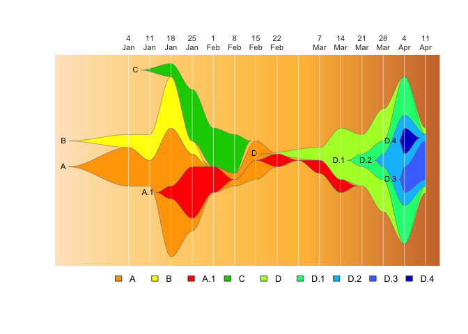
fishPlot(epifish_output$fish, shape="spline",
         vlines=epifish_output$timepoints, vlab=epifish_output$timepoint_labels)
drawLegend(epifish_output$fish, nrow=1)
The fishplot package provides further flexibility in where to display the vertical lines and what text to show, which can be used to create custom combinations rather than using the epifish defaults:
If things are getting crowded, you can label just every other week:
#subset timepoints and labels to ever other entry
vlines <- epifish_output$timepoints[c(TRUE, FALSE)]
vlabs  <- epifish_output$timepoint_labels[c(TRUE, FALSE)]

fishPlot(epifish_output$fish, shape="spline", vlines=vlines, vlab=vlabs)Or add a “zero” timepoint with the first case, which starts on the fourth day of the first epi week (we’ll also make the text a bit smaller so it doesn’t overlap):
vlines <- c((4/7), epifish_output$timepoints)
vlabs <- c("1\nJan", epifish_output$timepoint_labels)

fishPlot(epifish_output$fish, shape="spline",
vlines=vlines, vlab=vlabs, cex.vlab=0.5)We can specify completely custom timepoints and labels that describe an epidemiological story, with red lines:
vlines <- c((4/7), 3, 8.5, 14)
vlabs <- c("first\ncases", "wave 1", "quarantine\nbreach", "wave 2")

fishPlot(epifish_output$fish, shape="spline",
vlines=vlines, vlab=vlabs, col.vline="red")You can modify how far back in time the clusters seem to “begin” using
the pad_left argument to fishplot::fishPlot():
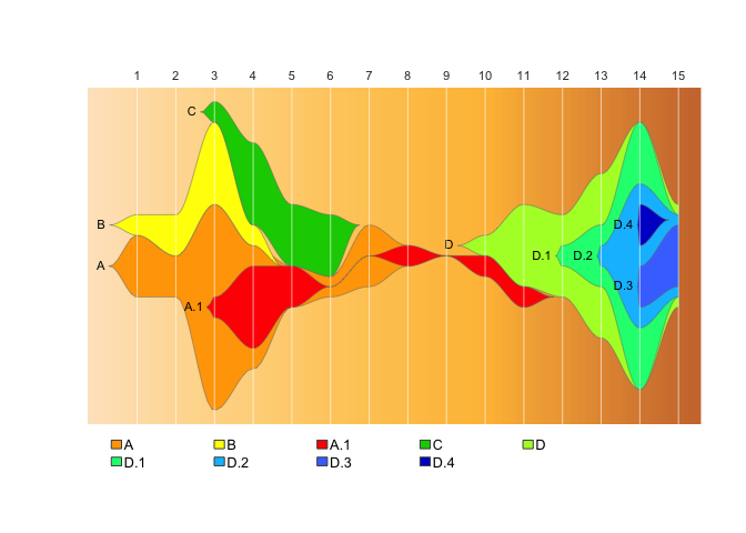
fishPlot(epifish_output$fish, shape="spline", vlines=epifish_output$timepoints, vlab=epifish_output$timepoint_labels,  pad.left=0.05)
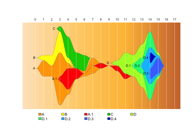
drawLegend(epifish_output$fish, nrow=2, widthratio=0.3, xsp=0.2)You can add extra “padding” timepoints to the start and end of the data
using the start_time and end_time arguments of
epifish::build_epifish:
epifish_output <- build_epifish (sample_df, parent_df, colour_df, start_time = 0, end_time = 17)
#> Checking for missing timepoints:
#>  - Adding zero counts for missing timepoint: 0
#>  - Adding zero counts for missing timepoint: 9
#>  - Adding zero counts for missing timepoint: 16
#>  - Adding zero counts for missing timepoint: 17
#> setting parent position of child A.1  to  1
#> setting parent position of child D.3  to  7
#> setting parent position of child D.2  to  6
#> setting parent position of child D.1  to  5
#> setting parent position of child D.4  to  7
#> Padding parent values in matrix:
#> adding child  D.4  to parent  D.2
#> adding child  D.3  to parent  D.2
#> adding child  D.2  to parent  D.1
#> adding child  D.1  to parent  D
#> adding child  A.1  to parent  A
#> The maximum sample count per timepoint (height of Y-axis) is:  15

fishPlot(epifish_output$fish, shape="spline", vlines=epifish_output$timepoints, vlab=epifish_output$timepoint_labels,  pad.left=0.05)
drawLegend(epifish_output$fish, nrow=2, widthratio=0.3, xsp=0.2)Using fishplot v0.5.1+, you can modify the spacing of the epi-fishplot
legend, which is especially useful with long cluster names. Use
widthratio to adjust the width between columns relative to the longest
cluster name (smaller value = more space), and xsp to control space
between the colour box and the text (larger = more space)
fishPlot(epifish_output$fish, shape="spline", vlines=epifish_output$timepoints, vlab=epifish_output$timepoint_labels)
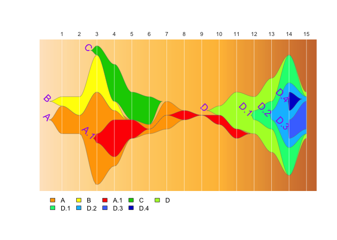
drawLegend(epifish_output$fish, nrow=2, widthratio=0.3, xsp=0.2)Using fishplot v0.5.1+, you can modify the size, colour, position, and
angle of cluster labels when building fishplot objects. You can set
these values using arguments to epifish::build_epifish().
epifish_output <- build_epifish(sample_df, parent_df, colour_df,
                                label_col = "purple",
                                label_angle = -45,
                                label_cex = 1.2,
                                label_pos=2,
                                label_offset=0.05)
#> Checking for missing timepoints:
#>  - Adding zero counts for missing timepoint: 9
#> setting parent position of child A.1  to  1
#> setting parent position of child D.3  to  7
#> setting parent position of child D.2  to  6
#> setting parent position of child D.1  to  5
#> setting parent position of child D.4  to  7
#> Padding parent values in matrix:
#> adding child  D.4  to parent  D.2
#> adding child  D.3  to parent  D.2
#> adding child  D.2  to parent  D.1
#> adding child  D.1  to parent  D
#> adding child  A.1  to parent  A
#> The maximum sample count per timepoint (height of Y-axis) is:  15
fishPlot(epifish_output$fish, shape="spline", vlines=epifish_output$timepoints, vlab=epifish_output$timepoint_labels,  pad.left=0.05)
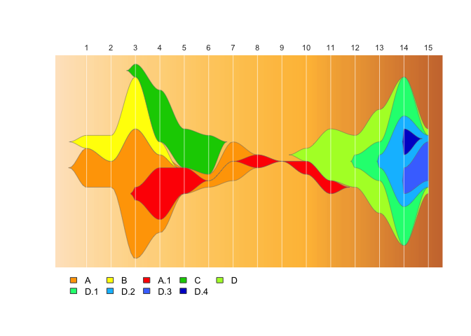
drawLegend(epifish_output$fish)If you don’t want to show the cluster labels on the fishplot, set
label_clusters=FALSE in epifish::build_epifish().
epifish_output <- build_epifish (sample_df, parent_df, colour_df, label_clusters=FALSE)
#> Checking for missing timepoints:
#>  - Adding zero counts for missing timepoint: 9
#> setting parent position of child A.1  to  1
#> setting parent position of child D.3  to  7
#> setting parent position of child D.2  to  6
#> setting parent position of child D.1  to  5
#> setting parent position of child D.4  to  7
#> Padding parent values in matrix:
#> adding child  D.4  to parent  D.2
#> adding child  D.3  to parent  D.2
#> adding child  D.2  to parent  D.1
#> adding child  D.1  to parent  D
#> adding child  A.1  to parent  A
#> The maximum sample count per timepoint (height of Y-axis) is:  15

fishPlot(epifish_output$fish, shape="spline", vlines=epifish_output$timepoints, vlab=epifish_output$timepoint_labels,  pad.left=0.05)
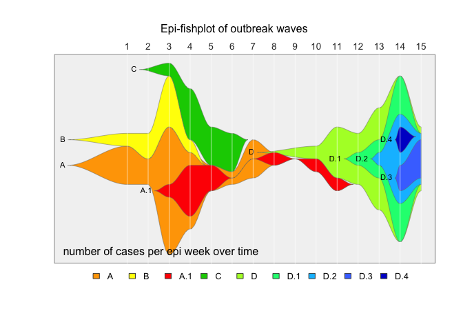
drawLegend(epifish_output$fish)You can also adjust assorted aspects of the fishplot as arguments to
fishplot::fishPlot(). For details, refer to the documentation for the
fishplot package (try the command ?fishplot::fishPlot).
epifish_output <- build_epifish(sample_df, parent_df, colour_df)
#> Checking for missing timepoints:
#>  - Adding zero counts for missing timepoint: 9
#> setting parent position of child A.1  to  1
#> setting parent position of child D.3  to  7
#> setting parent position of child D.2  to  6
#> setting parent position of child D.1  to  5
#> setting parent position of child D.4  to  7
#> Padding parent values in matrix:
#> adding child  D.4  to parent  D.2
#> adding child  D.3  to parent  D.2
#> adding child  D.2  to parent  D.1
#> adding child  D.1  to parent  D
#> adding child  A.1  to parent  A
#> The maximum sample count per timepoint (height of Y-axis) is:  15
fishPlot(epifish_output$fish, shape="spline",
         vlines=epifish_output$timepoints,
         vlab=epifish_output$timepoint_labels,
         pad.left=0.2,
         cex.vlab=0.85,
         title="Epi-fishplot of outbreak waves",
         title.btm="number of cases per epi week over time",
         cex.title=1,
         bg.type="solid",
         bg.col="grey95")
#> [1] "WARNING: there were not 3 background gradient colors set - falling back to defaults"
drawLegend(epifish_output$fish, nrow=1, xpos=-1)If you use epifish in your work, please cite:
- epifish: Documenting elimination of co-circulating COVID-19 clusters using genomics in New South Wales, Australia. Arnott A, Draper J et al. BMC Research Notes. 10.1186/s13104-021-05827-x
- fishplot: Visualizing tumor evolution with the fishplot package for R. Miller CA, McMichael J, Dang HX, Maher CA, Ding L, Ley TJ, Mardis ER, Wilson RK. BMC Genomics. doi:10.1186/s12864-016-3195-z
See also:
citation("epifish")This work extends the Chris Miller’s fishplot package
(https://github.com/chrisamiller/fishplot). It was written by
Dr. Jenny Draper, a member of the pathogen genomics team employed by
New South Wales Health
Pathology, at the Westmead
Hospital Institute of Clinical Pathology & Medical Research (ICPMR)
Centre for Infectious Diseases and Microbiology - Public
Health
in Australia. epifish was initially developed as part of the NSW
government’s response to COVID-19.

