We consider a generalization of stochastic bandits where the set of arms, X, is allowed to be a generic measurable space and the mean-payoff function is “locally Lipschitz” with respect to a dissimilarity function that is known to the decision maker. Under this condition we construct an arm selection policy, called HOO (hierarchical optimistic optimization), with improved regret bounds compared to previous results for a large class of problems. In particular, our results imply that if X is the unit hypercube in a Euclidean space and the mean-payoff function has a finite number of global maxima around which the behavior of the function is locally continuous with a known smoothness degree, then the expected regret of HOO is bounded up to a logarithmic factor by √n, that is, the rate of growth of the regret is independent of the dimension of the space.¹
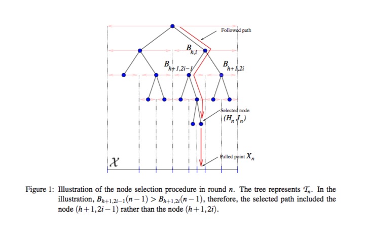
The HOO strategy incrementally builds an estimate of the mean-payoff function f over X. The core idea is to estimate f precisely around its maxima, while estimating it loosely in other parts of the space X. To implement this idea, HOO maintains a binary tree whose nodes are associated with measurable regions of the arm-space X such that the regions associated with nodes deeper in the tree represent increasingly smaller subsets of X. The tree is built in an incremental manner. At each node of the tree, HOO stores some statistics based on the information received in previous rounds. In particular, HOO keeps track of the number of times a node was traversed up to round n and the corresponding empirical average of the rewards received so far. Based on these, HOO assigns an optimistic estimate (denoted by B) to the maximum mean-payoff associated with each node. These estimates are then used to select the next node to “play”. This is done by traversing the tree, beginning from the root, and always following the node with the highest B-value. Once a node is selected, a point in the region associated with it is chosen and is sent to the environment. Based on the point selected and the received reward, the tree is updated.²
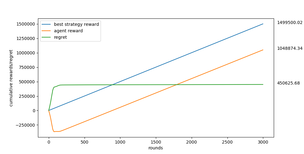 Figure 1: Results of the bandit algorithm where the reward function = 500 - Σi(xᵢ-i)² where Σ is from 1 to 10.
Hence X-space is 10 dimensional while each dimension's range is [-60,60].
 Figure 2: The last selected arm is the most rewarding point in the 10-dimensional X-space that is discovered so far.
Each dimension's range was [-60,60]. Notice that the global maxima is 500 when x = (1,2,3,4,5,6,7,8,9,10) which the bandit approximated well in 3000 rounds.
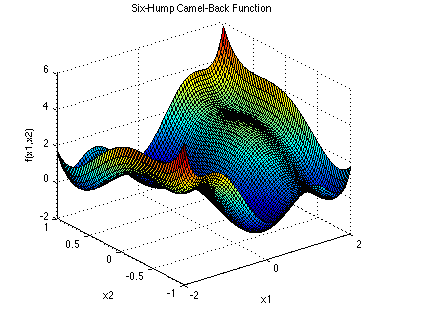
Figure 3: Six-hump camelback function. A widely used global optimization function. It has two global minumum at (x1,x2) =(-0.0898,0.7126), (0.0898,-0.7126), and multiple local minima.
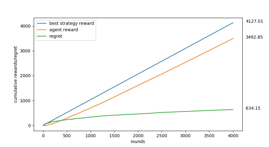 Figure 4: Results of the bandit algorithm where the reward function = -six_hump_camelback function.
The dimensions were constrained to be [-2,2] and [-1,1] as in Figure 3.
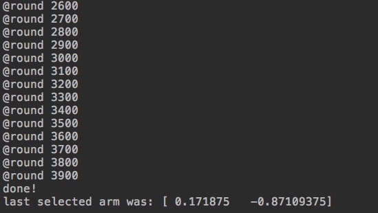
Figure 5: The last selected arm is the most rewarding point in the 2-dimensional X-space that is discovered so far. Even though the bandit has not yet discovered the global maximum, it has gotten very close to it in 4000 rounds.
import Partitioner
import TestFunctions
import HOO

    # choose a test function.
    testFunction = TestFunctions.TestFunctions(functionName="hyper_ellipsoid", dimensions=10)
    # testFunction = TestFunctions.TestFunctions(functionName="analytical_g", g_params=np.array([0.1, 0.3, 1, 3, 10, 30, 90, 300]))
    # testFunction = TestFunctions.TestFunctions(functionName="SixHumpCamelback")

    #  get the min and max bounds of the domain of the test function.
    bounds = testFunction.get_bounds()

    # initialize a partitioner that will generate the tree covering sequence from the space-X defined by the above "bounds."
    partitioner = Partitioner.Partitioner(min_values=bounds[0], max_values=bounds[1])

    # initialize the bandit algorithm with the following.
    # ro = 0.5 is generally a good choice, for symmetric or near-symmetric X-spaces.
    #  a good choice of v1 would be >= dimensions*6 for "hyper_ellipsoid function",
    # and >= 6 for "analytical_g" and "sixhumpcamelback"

    x_armed_bandit = HOO.HOO(v1=60, ro=0.5, covering_generator_function=partitioner.halve_one_by_one)
    x_armed_bandit.set_time_horizon(max_plays=1000)
    x_armed_bandit.set_environment(environment_function=testFunction.draw_value)
    x_armed_bandit.run_hoo()

    # this is the most rewarding point explored so far after "max_plays" rounds.
    print ("last selected arm was: {0}".format(x_armed_bandit.last_arm))

    # the rewards that are received by the bandit should be stored by the environment, as well as the best-fixed strategy.
    rewards = testFunction.drawn_values
best = testFunction.bests¹ ² S. Bubeck, R. Munos, G Stoltz, and C. Szepesvari. X-armed Bandits. Journal of Machine Learning Research 12 (2011) 1655-1695, 2011.
