Repository to reproduce the analyses in the paper “Diurnal temperature range as a key predictor of plants’ elevation ranges globally”.
Simply use the main.R file to run all the analyses performed in the
manuscript.
You can run multiple models automatically using a set of for loops.
For example:
# global-scale analyses

model <- load_model(scope = "global")

for (expr in c(~dtr, ~ts, ~past_dmat)) {
  for (elevation_span in ELEV_SPANS) {
    for (exclusion_zone in EXCLS) {
      mdl_data <- compile_mdl_data(
        trs,
        clim_data = trs_bioclim,
        elevation_span = elevation_span,
        exclusion_zone = exclusion_zone,
        singleton_thr = SINGLETON_THR,
        std_elev_grad = TRUE,
        average = TRUE,
        std_from = "top",
        cols = c("location", "sp_range", "land_type"),
        expr = expr
      )

      run_jags(
        mdl_data,
        model = model,
        n.iter = JAGS_ITER,
        n.thin = JAGS_THIN,
        n.chains = JAGS_CHAINS,
        n.burnin = JAGS_BURN_IN,
        save = TRUE,
        path = glue("data/jags/{model$scope}-scale/")
      )

      gc() # to free up RAM
    }
  }
}
Note that the expr parameter in compile_mdl_data() takes a
formula for the global-scale analyses and a character string for
the local-scale analyses.
A list of the different models ran in the manuscript can be found below.
Once the models have finished running, use:
results.Rto plot model estimates and get model statisticsmdl_diagnostics.Rto perform model diagnostics
- Global-scale analyses:
- main models:
~dtr,~ts,~past_dmat - land type:
~dtr * land_type,~ts * land_type,~past_dmat * land_type - climate-related interactions:
~dtr * ap,~dtr * mat,~past_dmat * past_map
- main models:
- Local-scale analyses:
"dtr","ts"
Run the following line to make the required data set to reproduce the analyses on Gilchrist’s hypothesis.
trs_dtr_lower_third <- filter(trs, bio2 <= max(bio2, na.rm = TRUE) / 3)Run the ~past_dmat model using the trs_dtr_lower_third data set.
model <- load_model(scope = "global")

for (elevation_span in ELEV_SPANS) {
  mdl_data <- compile_mdl_data(
    trs_dtr_lower_third,
    clim_data = trs_bioclim,
    elevation_span = elevation_span,
    exclusion_zone = EXCL_DEFAULT,
    singleton_thr = SINGLETON_THR,
    std_elev_grad = TRUE,
    average = TRUE,
    std_from = "top",
    cols = c("location", "sp_range", "land_type"),
    expr = ~past_dmat
  )

  run_jags(
    mdl_data,
    model = model,
    n.iter = JAGS_ITER,
    n.thin = JAGS_THIN,
    n.chains = JAGS_CHAINS,
    n.burnin = JAGS_BURN_IN,
    save = TRUE,
    path = "data/jags/global-scale/gilchrist hypothesis/"
  )
}
Use the GlobalAnalyses class to plot model estimates:
gh <- GlobalAnalyses$new("data/jags/global-scale/gilchrist hypothesis")

gh$regressions(
  vars = "past_dmat",
  facet_cols = "elevation_span",
  labels = "∆ mean annual temperature (0-1980) (°C)"
)

gh$posterior_distributions(
  vars = "past_dmat",
  yvar = "elevation_span",
  facet = FALSE,
  reverse = TRUE,
  scales = .6
)
Climate data are already provided in the trs.csv data set.
If you would like to perform GIS analyses again, proceed as follows:
- Open
TRS.Rprojand execute the following function in the console:TRS.utilities::setup_gis(). The function will create all the required directories to store SRTM and climate-related data. - Download bioclim and
digital elevation data (as
.tif) as well as PaleoView. See here for instructions to generate past climate data. - Save each file in the appropriate folder (see file tree below).
- Once all the files are in their respective folders, use the
gis.Rscript to extract present and past climate data in each location. Output data will be stored in thegis/clim/extracted/subfolders.
gis
├── clim
│   ├── data
│   │   ├── past                        <- PaleoView-related folder
│   │   │   ├── base                    <- past climate data go here
│   │   │   └── var
│   │   │       ├── mean precipitation  <- generated mean precipitation files go here
│   │   │       └── mean temperature    <- generated mean temperature files go here
│   │   └── present                     <- present bioclim files go here
│   └── extracted
│       ├── past
│       └── present
└── srtm                                <- save SRTM tiles in the corresponding subfolders
    ├── Afghanistan
    ├── Alborz Mountains
    ├── Azores
    ├── Baekdudaegan Mountains
    ├── Bioko
    ├── Canary
    ├── Cantabria
    ├── Cape Verde
    ├── Chicauma
    ├── Colombian Andes
    ├── Crete
    ├── Cyprus
    ├── Denali
    ├── Drakensberg
    ├── Euboea
    ├── Golestan
    ├── Hawaii
    ├── Hengduan
    ├── Jamaica
    ├── Jaya
    ├── Kenya
    ├── La Amistad
    ├── Lazio
    ├── Mt Ararat
    ├── Mt Etna
    ├── Mt Kilimanjaro
    ├── Nanga Parbat
    ├── Nepal
    ├── Nevada Test Site
    ├── Owens Peak
    ├── Reunion
    ├── Santa Rosa Mountains
    ├── Sierra Nevada
    ├── Sierra San Pedro Martir
    ├── Socotra
    ├── South-Eastern Pyrenees
    ├── Swiss Alps
    ├── Tahoe
    ├── Taiwan
    ├── Tajikistan
    ├── Tasmania
    ├── Utah
    ├── Venezuelan Andes
    └── Wind River Mountains
Open PaleoView and download the climate data (see chapter 2 of
PaleoView’s user
manual)
for mean temperature and precipitation. Configure the input data
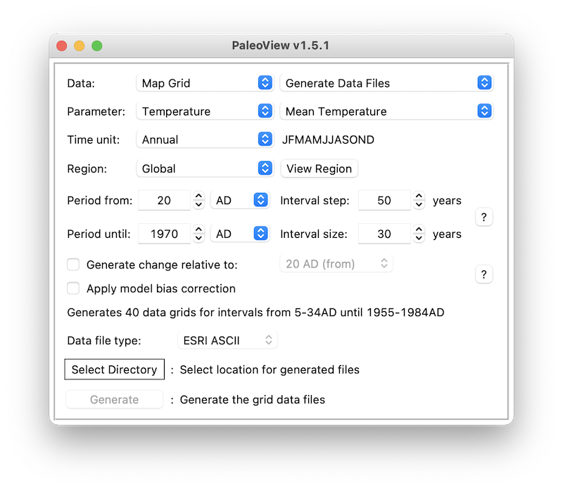
location (see chapter 3 in the user manual). Run PaleoView with the same
settings as shown in the image below for temperature and
precipitation:
Below are the different R packages required to run the code in this repository:
- tidyverse
- TRS.utilities
- glue
- bayesplot (only for model diagnostics)
To install TRS.utilities, use:
# install.packages("pak")
pak::pak("arnaudgallou/TRS.utilities")
In addition, you will need to have JAGS installed on your machine.
